Few measurements are as prevalent as that of temperature. While sometimes it is of primary interest, knowledge of temperature is often a parameter used to compensate for its effects on other measurements. Radio frequency amplifiers, mixers, and other components are examples of temperature-dependent circuits; photodiodes and avalanche photodiodes are another. In more challenging applications, both high accuracy and dynamic range are desirable for temperature measurements.
A bridge circuit using a thermistor can provide high accuracy, but is limited to a small dynamic range. The simple voltage divider circuit we describe in this article gives the design engineer the ability to achieve a wide range of temperature measurements with good accuracy, yielding three sigma (3σ) errors in the range of 0.2°C to 0.35°C, as in Figure 1. To achieve better performance, you can calibrate off-the-shelf thermistors or have this done by the manufacturer to achieve accuracies in the milliKelvin (mK) range. The combination of a low component count, wide dynamic range, and high accuracy make this circuit useful to a broad range of target applications. Choosing small thermistors also results in minimal lag in the measurement due to their low thermal mass, an important characteristic in rapidly changing thermal environments.
Figure 1 presents the 3σ absolute accuracy of our simple circuit. The circuit's original application was to provide temperature compensation information for a photodiode-based instrument—the GOES-R X-ray spectrometer, which measures the intensity and location of solar flares, as well as the solar minimum background X-ray irradiance—capable of accurately measuring currents in the tens of femtoAmps range. In this application, the ability to track relative changes in temperature was more important than absolute accuracy. We found the relative accuracy of the circuit to be approximately ten times better (0.04°C) than its absolute accuracy. The Laboratory for Atmospheric Space Physics at the University of Colorado, contracted to have a low-noise, low-power charge electrometer ASIC developed for measuring photocurrent to 10 fA resolution and over a range from 50 fA to 10 nA. During testing, it was discovered that the offset voltage generated by the electrometer amplifier, in combination with the exponentially temperature-dependent shunt resistance of the photodiode in the instrument, generated a significant change in the circuit's quiescent current. Figure 2 shows the relationship between the baseline current and temperature, which looks linear because of the logarithmic vertical axis.
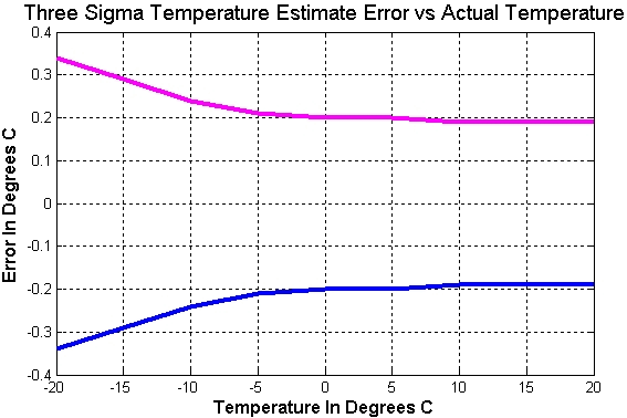 Figure 1. 3σ error bounds in estimating temperature when using Monte Carlo analysis for the circuit shown in Figure 3 |
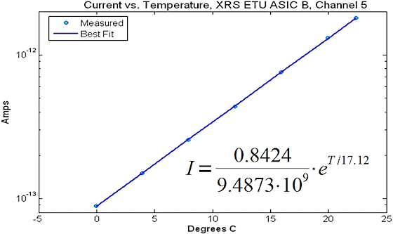 Figure 2. The exponential photodiode baseline current vs. temperature for the LASP X-Ray Spectrometer instrument |
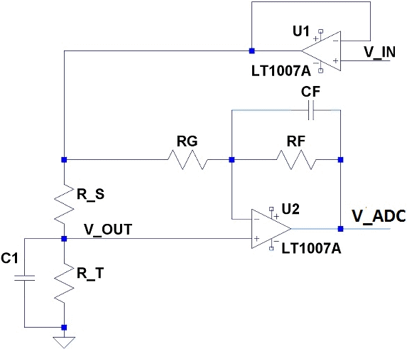 Figure 3. Schematic of the temperature monitoring circuit |
The circuit for monitoring temperature is shown in Figure 3. Using a series resistor, RS, with a thermistor, RT, the output voltage is given by Equation 1:
|
|
(1) |
where:
| VADC | = | output voltage |
| VI | = | input voltage |
| RS | = | a series resistor |
| RT | = | a thermistor |
| RF, RG | = | gain setting resistors with gain G, given by Equation 1a: |
 |
(1a) |
For maximum linearity, we need the rate of change of voltage vs. temperature, T, to be equal for both the minimum (Tmin) and maximum (Tmax) desired operational temperatures. That is, Equation 2 must be true for T = Tmax and T = Tmin of the measurement range:
 |
(2) |
The value of RS that yields the best linearization is solved from the second-order equation shown as Equation 3:
 |
(3) |
where:
| TT1 | = | lowest circuit operational temperature |
| RT1 | = | thermistor resistance at TT1 |
| TT3 | = | highest circuit operational temperature |
| RT3 | = | thermistor resistance at TT3 |
Figure 4. Thermistor temperature and resistance values at operational temperature limits of ±32°C
| Temperature (°C) | Thermistor Resistance (KΩ) |
| –32 | 151.2 |
| –31 | 143 |
| 0 | 29.49 |
| 31 | 7.88 |
| 32 | 7.58 |
The derivatives in Equation 3 can be solved using a table of thermistor resistance vs. temperature, using the two values closest to TT1 and TT3. At the limits of ±32°C, from Figure 4 we get the results below:

Substituting these values into Equation 3, the value of RS that gives us the best linearizing resistance is RS =26.459 KΩ. Another, simpler method is to choose RS = RTO, where RTO is the thermistor resistance at the middle of the desired operational temperature range. For example, RTO at T = 0°C is 29.49 KΩ. The result of both of these methods is shown in Figure 5. The rate of change of voltage vs. temperature is explicitly stated for the two limits of temperature operation, and the dV/dT values are very close to the same value at the temperature extremes. This means that we are obtaining a circuit response that is as close to linear as possible.
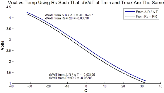 Figure 5. Voltage vs. temperature plot generated using the RS value that maximizes linearity (blue), and using RS = midpoint RTHERMISTOR, or RTHERMISTOR at 0°C (black line) |
While providing good linearization, the result does not span the desired range of VMIN to VMAX. However, if we can choose a gain and offset we can achieve this. The first step is to find VO for RT = RT1 (lowest temperature and highest resistance) and for RT = RT3 (highest temperature and lowest resistance) using Equations 4 and 5:
 |
(4) |
 |
(5) |
where:
| VIN | = | input voltage to the circuit (see Figure 3) |
| RS | = | series input resistance in the circuit (see Figure 3) |
| VOMAX | = | max. divider circuit voltage, which is the voltage at the thermistor for the lowest temperature and highest resistance, producing the max. circuit voltage |
| VOMIN | = | min. divider circuit voltage, which is the voltage at the thermistor for the highest temperature and lowest resistance, producing the min. circuit voltage |
Now set the circuit minimum and maximum voltages (VADCMIN and VADCMAX, respectively) at the temperature limits. Make VADCMIN = 0 and VADCMAX = VMAXADC, which is the max. voltage of the ADC using gain G and offset voltage VOFF as we see in Equations 6 and 7:
 |
(6) |
 |
(7) |
Through substitution we get Equations 8 and 9:
 |
(8) |
 |
(9) |
Equation 10 gives the output voltage of the circuit:
 |
(10) |
Figure 6 shows the voltage vs. temperature behavior for a circuit with VADCMAX = 4.096, VIN = 4.096, G = 1.5973, VOFF = –1.5099, and temperature range from ±32°C. The line is close to linear. The near constant slope, dV/dT, means that the output of an ADC will have a near constant change in counts vs. temperature, dN/dT, ensuring near-equal sensitivity across the chosen range of temperatures. At this point, we could analyze the error due to the amount of nonlinearity in the curve, assuming that the voltage follows the equation V =cT +VO . Alternatively, because there are two inflection points, we could minimize the error by fitting a third-order polynomial to the result. A better option, however, is to employ the Steihnhart-Hart Equation (SH-H) shown in Equation 11.
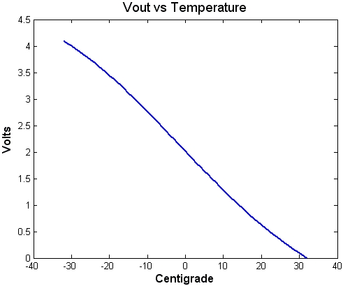 Figure 6. Voltage vs. temperature plot generated using a resistor divider and with gain and offset to span 0 to 4.096 V |
 |
(11) |
The use of SH-H involves solving Equation 10 for the resistance of the thermistor, RT, given a measured voltage VADC, and plugging this value into Equation 11 to solve for temperature. RT is calculated using Equation 12:
 |
(12) |
The coefficients a, b, and c in SH-H are solved using three points from the resistance vs. temperature table of the desired thermistor using Equation 13:
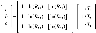 |
(13) |
where:
| RT1, RT2, RT3 | = | thermistor resistance at temperatures T1, T2, T3 |
| T1, T2, T3 | = | temperature in degrees Kelvin. |
We will not be discussing the best choices of T1, T2, and T3 here. Instead, our approach is to choose T1 as the lowest temperature to be measured, T3 as the highest temperature to be measured, and make T2 the midpoint of T1 and T3.
Figure 7 shows the errors in estimating temperatures between ±32°C using the two methods. The blue line is the error when using SH-H to estimate temperatures over our temperature range; the maximum error is 0.012°C. The green line is the error when we estimate temperature using a third-order polynomial fit; the maximum error is 0.21°C. When we compare the two results we find that the error using SH-H vs. the error using the polynomial fit is 18.6 times smaller. Using a seventh-order polynomial fit will work slightly better than using SH-H over the range of ±30°C; however if we increase the temperature range to ±50°C, the SH-H equation again does a much better job of estimating the temperature. Thus, by using SH-H we no longer need to determine the polynomial order required to get an accurate temperature measurement over a large range of temperatures.
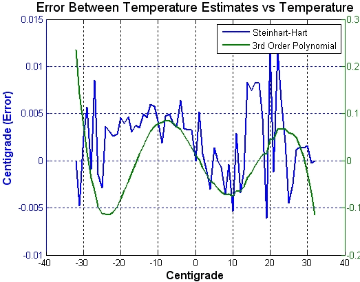 Figure 7. Estimated temperature errors using the Steinhart-Hart equation (blue line) and a third-order polynomial (green line) |
In part two of this article, we'll apply these methods and show how, by characterizing the thermistors' behavior in a thermal bath, we can use the combination to achieve high-accuracy temperature readings over a wide range.
ABOUT THE AUTHORS
Darren O'Connor is an Electrical Engineer at the Laboratory for Atmospheric and Space Physics, University of Colorado, Boulder, CO. He can be reached at [email protected].
Kasandra O'Malia is a Calibration Engineer at the Laboratory for Atmospheric and Space Physics, University of Colorado, Boulder, CO. She can be reached at [email protected].
