

Embedded software for sensor applications presents its own particular set of development challenges. It is not uncommon for a sensor application to require high-speed reaction, memory capacity, and a compact design to maintain a small physical footprint. Sensors that are remotely located and battery powered also need to deliver the longest possible operation on a charge. Such performance is not just a matter of hardware—software can also play an important role. Whether or not you are a software developer, understanding the tools and techniques used to optimize the size, speed, and power efficiency of the code in a device will help you minimize its power footprint and maximize its battery life.
Intelligent sensors are sensors that incorporate a low-power microcontroller unit to read data from the sensor and to communicate with other nearby intelligent sensors. For example, a series of intelligent sensors to detect chemical, biological, and radioactive threats could be deployed around sensitive areas such as sporting events or government buildings. If one sensor detects a threat, it passes that information on to the other sensors and, through the chain to a central command station. While any low-power microcontroller can provide the intelligence of an intelligent sensor, this article will assume that you are using an ARM Cortex-M3 microcontroller. However, the software optimization techniques we discuss can be applied to many different kinds of microcontroller architectures.
Modular design doesn't just benefit hardware platforms. The surest way to arrive at the best possible product is to start by organizing the project in a way that makes the software easy to optimize, debug, and maintain. By using this type of top-down approach, it is easier to develop new intelligent sensors based on your old designs or, alternatively, to add new kinds of intelligent sensors to existing networks. Your team can do this by dividing your source code into different source code groups. You might, for example, put the communications firmware in one group; knowing where to look for the source code that handles a specific task or part of the application makes the application as a whole easier to maintain. This method lends itself to generating a code block or library of that part of the code that can be reused for other applications that use the same communication hardware. It makes debugging easier and allows you to lower or raise the optimization level for a group of source files. Arranging all source files for a specific functionality in the same group gives the compiler freedom to more effectively optimize all of the code in that group in one chunk, otherwise known as multi-file compilation.
Now that we have some structure in our project, how do we optimize the use of resources such as battery and processing power and the cost to develop the sensors? To minimize both the code footprint and cost of the device, we should use as little memory as possible. The smaller the program, the smaller the amount of memory required to store it. Compilers typically have optimization capabilities to assist with this, but these capabilities vary from compiler to compiler.
For best results the compiler needs to be able to perform high-level optimizations and to be core specific; e.g., offering low-level optimizations for the different Cortex-M cores. Without these capabilities, the generated code will not be well optimized for your device. For example, we can set the compiler's project level optimization to optimize for size. The reduction in the size of the generated code will differ from application to application, but typical reductions from this step can run from 10% to 20%.
Applications that require initialization of variables and arrays located in nonpersistent (volatile) memory can further reduce memory usage. If we let our linker (which creates the final image to be downloaded) compress the values used to initialize an array, we might see size reductions of up to 90% or more in the code/constants (const) memory space. This technique requires adding an unpacking (decompressing) algorithm to the application, but the reduction in the code size can still be significant for some applications, as we can see in the chart in Figure 1. Initializers assign initial values to variables and data structures and are executed during the device's startup. By using a compressed initializer these initialization data are 'zipped' (compressed) and then unzipped by the startup code. This process can reduce the size of the initialization code by 90% and reduce the size of the generated application code by about 15%.
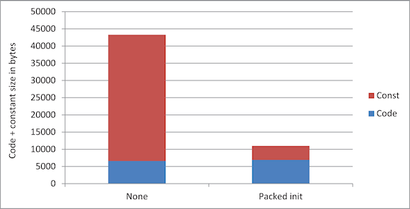 Figure 1. Using initialization optimization and an unpacking algorithm can drop the number of bytes required for constants (brick color) and for the code itself (blue) by up to 90% |
For further savings, we can use either RAM or flash memory for both function and data storage. For our example intelligent Cortex-M-based sensor, we had a large array that was located in RAM and initialized from compressed values located in our flash memory. If we were short of RAM we could, in the compiler, load our array into the memory allocated for const provided, of course, that it was an array of constants.
We can do the same with functions, determining whether they should be located and executed in RAM or flash memory. This gives us the flexibility to locate functions where we still have unused memory and gives us speed optimization because functions usually execute faster in RAM than they do when executing out of flash memory.
Speed Up!
Now that we have decreased the footprint of our application software we will focus on adding speed to functions that must meet timing requirements. The first step is to identify the code segments that need extra speed. Armed with that information, we can override the size optimization for those functions and have the compiler optimize them for speed. Optimizing for both size and speed can provide big advantages in overall resource usage, as we see in Figure 2.
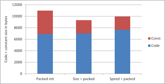 Figure 2. Bars show the code + const size for compressed initializers for different compiler optimization settings |
The profiling tool in the debugger allows you to see how many times different parts of the code have been executed, which helps you identify code blocks where speed optimization might have a big impact on the overall performance. The methods used for measuring the execution speed and the time spent in different parts of the code depend heavily on your device and which debugger you have used. If your debugger supports instruction trace, for example, then you could start the trace at one location in the code and stop it at another. The trace view would then contain information on when trace started and stopped, allowing you to calculate the time spent between these two points in the code. Other techniques for measuring the time spent in different parts of the code include setting breakpoints or adding print statements.
Normally we compile each file separately. This prevents the compiler from making some optimizations that would be possible if it had some information about the rest of the system. If the compiler supports multi-file compilation, then we can feed the compiler with more information about our system and get a better result from optimization steps. We can, in fact let the compiler compile all our C/C++ code in one compilation. This is an option for smaller projects but in larger projects this might involve compiling thousands or tens of thousands of source files at once, which could be very time-consuming. Therefore, for larger projects it is better to apply this technique to subsets of associated files.
Power Optimization
After optimizing our design for both code size and execution speed, now let's consider ways to reduce power consumption. We can do this by changing the code structure and modifying the compiler optimization settings. Consider an application that measures and displays the temperature every 10 s, for example. We could model some different scenarios, such as turning off other peripherals during data capture, but that might turn out to be hard to do or overlook unknown factors. For instance, the output of one sensor may depend on the output of another sensor. Or there may be multiple developers working on a project, each of whom is responsible for monitoring a different sensor. If one developer shuts off a microcontroller peripheral it may have unexpected results because the other developer may expect that peripheral to remain always on. A better solution is power debugging, which involves evaluating power consumption during code execution and tracing spikes in consumption back to specific lines of code. This approach can also uncover unsuspected 'power bugs'; an IO port that is set up incorrectly, for example, might drain the system of power. Such a problem would be easily found if we have information about the power consumption during the execution of the application.
For instance, IAR Embedded Workbench, an integrated compiler, assembler, linker, and debugger software tool suite, features a Timeline Window that provides an overview of the system power consumption (Figure 3). Notice that the power consumption goes up just after 1.85 s—to find out why, we can double-click on that part of the graph and the debugger takes us to the location in the code where this happened. The function profiler allows us to view the power consumption for each function in our system (Figure 4). This helps us understand which functions are consuming the most energy so that we can adjust overall performance, maybe by optimizing some of these functions for speed rather than size.
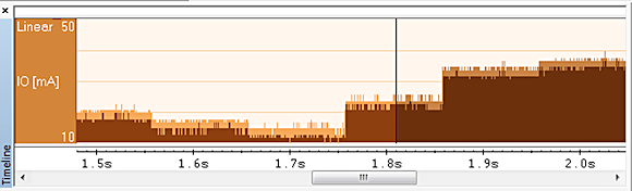 Figure 3. Timeline Window in IAR Embedded Workbench reveals periods of high power consumption, which can be traced back to the source code |
 Figure 4. The Function Profiler window in IAR Embedded Workbench displays the energy and current consumption by the device under test in different parts of the code |
There are many more things you can do to reduce your application's power consumption. For example, you could take advantage of any low-power modes that your device might have. Using timers instead of delay loops also provides big benefits—delay loops usually consume a lot of power, so setting up a timer to count down and then entering a low-power mode while waiting for the timer to trigger is much more efficient. If you use a real-time operating system (RTOS), reducing power consumption during idle time is a great way to extend battery life. And as a last tip, the higher the frequency at which the device runs, the more power it will consume, so look for parts of your application where you can lower the CPU frequency to reduce the power consumption.
Although many of the constraints in sensors—size, cost, speed—tend to be hardware-oriented, optimizing software plays an essential role in the performance of the final product. By applying the different types of optimization in the order described above, your team can more rapidly deliver to market a device that meets specifications.
RESOURCES
For more information about optimization and debugging techniques used in the article, see the IAR Systems Resource page.
To learn more about Cortex-M debugging features, see:
ABOUT THE AUTHOR
Mats Pettersson is U.S. Field Application Engineer Manager for IAR Systems AB, Uppsala, Sweden. He can be reached at [email protected].