
The perennial challenge for sensor interface designers is to calibrate and correct the inherent nonidealities present in transducers. The major contributors to nonideality are typically the nonlinear response to stimulus (gain), the offset, and the temperature dependence of one or both of these factors. Historically there have been myriad design approaches and solutions to this problem, but the advent of commodity ICs with high-performance analog and complex digital circuitry reduces the effort and cost of sensor correction and provides the designer with systematic methodologies and tools for sensor correction. This article examines these techniques and describes how to optimize them for one broad class of sensor signal conditioners (SSCs) that are inexpensive yet highly configurable, enabling high-precision measurements made using a range of sensor types. A vital part of this optimization is the expertise and development support provided by the SSC manufacturer.
Figure 1 is a block diagram of an SSC showing the typical sensor interface functionality for transducers that exhibit a time-invariant change in electrical properties in direct proportion to some physical stimulus. In this case, the sensor element is a Wheatstone bridge that changes resistance with respect to an input such as pressure or strain, but it could also be one of a variety of other transducers that experience a change in capacitance, voltage, or current in response to some input stimulus.
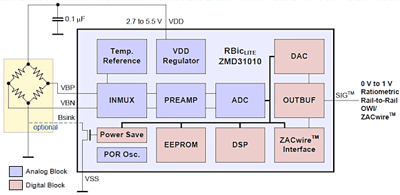 Figure 1. A representative example of an SSC that provides all the necessary functionality to condition and correct its sensor input |
The main functions of the SSC are to provide a bias source for the sensor, to amplify and possibly filter the sensor output(s), to digitize the amplified signal, to apply the appropriate correction factors based on pre-stored calibration coefficients, and to output the resulting linearized signal in digital or analog formats. The focus of this article is to explore in detail how the calibration coefficients are determined and applied using the predefined digital algorithms built in to the SSC.
Choosing an Appropriate Algorithm
The SSC in Figure 1 has ten different built-in algorithms from which the designer can choose. The challenges for the designer are how to choose and evaluate the most effective and efficient algorithm and then how to implement and test the calibration routine in a high-volume production environment. If the algorithm is too simplistic, system accuracy will suffer, and if it is unnecessarily complex, expensive and valuable test resources will be wasted acquiring superfluous calibration data with little or no benefit to system accuracy. In some cases, algorithms that are more complex can actually degrade accuracy, so choosing the right algorithm is very important.
As mentioned previously, the primary sources of sensor error are the offset and gain nonlinearity, and their variation over temperature. The first step in choosing a correction algorithm is to separate and quantify these effects. The designer must then evaluate how nonlinear they are with respect to sensor stimulus and temperature and determine the minimum level of correction necessary to meet system requirements.
Figure 2 is a list of the ten different algorithms for the SSC in Figure 1, organized by the type and degree of correction. Column two indicates, for each algorithm, how many measurement points are necessary to calculate the calibration coefficients. The number of measurement points is the same as the number of correction terms; it is important to recognize this because it shows the direct correlation between the level of correction and the measurement time required for calibration.
Figure 2. List of correction algorithms for the example SSC showing how many calibration points are necessary and what correction factors are applied
| Method | Number of points | Gain Linear | Gain Second Order | Gain TC Linear | Gain TC Second Order | Offset | Offset TC Linear | Offset TC Second Order | ||
| 1 | 2 | X | X | |||||||
| 2 | 3 | X | X | X | ||||||
| 3 | 3 | X | X | X | ||||||
| 4 | 3 | X | X | X | ||||||
| 5 | 4 | X | ||||||||
| 6 | 4 | X | X | X | X | |||||
| 7 | 4 | X | X | X | X | |||||
| 8 | 5 | X | X | X | X | X | ||||
| 9 | 5 | X | X | X | X | X | ||||
| 10 | 5 | X | X | X | X | X |
The columns in Figure 2 list which type of correction each calibration method applies; they also describe the sensor characteristics that must be isolated and quantified to determine the optimal algorithm. For clarity, these characteristics are divided between gain and offset parameters. This particular SSC allows up to second order correction for both gain and temperature coefficient (TC).
If you measure and plot gain and offset versus sensor stimulus at constant temperature, and then versus temperature with a constant input, you can observe these effects, analyze them separately, and evaluate them to see which calibration method contains the correction terms that correspond most closely to the observed sensor nonidealities. A pressure sensor, for example, would be characterized over its full input pressure range at 20°C and then over a wide temperature range with the input pressure fixed at 50% of maximum. In many cases, direct observation of plots like these will indicate quickly which calibration methods to consider or rule out. Referring to Figure 2, if a plot of offset versus temperature reveals that offset is constant with respect to temperature, then Methods 3, 5, 6, 8, and 10 should be eliminated immediately from consideration. At first glance it might seem that Method 9 could be eliminated, but if the gain TC is highly nonlinear, Method 9 might be required even though the offset TC is negligible. Further, if the gain is highly linear, Methods 2 and 7 could be removed from consideration. In this hypothetical case, the only algorithms remaining for evaluation would be Methods 1, 4, and 9, depending on the nonlinearity of the gain TC.
Creating a table such as this for an SSC with built-in calibration algorithms and then comparing the table with plots of measured sensor data can help you to quickly home in on the algorithms that need detailed quantitative evaluation. Inevitably, however, you will need to perform some detailed analysis of some or all of the algorithms to determine which of them is the most efficient for a particular system. Doing this manually can be tedious and time-consuming, and will require you to create some sort of spreadsheet or software to calculate and analyze the equations.
To get an idea of the level of effort required to evaluate a calibration algorithm, consider the first two methods in Figure 2. These are the simplest of the methods and do not include any temperature correction. Figure 3 shows the equations used in these two methods.
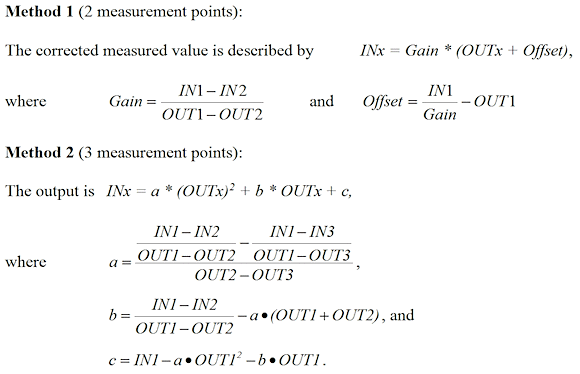 Figure 3. Equations used for the two simplest correction algorithms |
In the equations in Figure 3, IN1 and IN2 are known stimulus input values of pressure, force, tilt angle, etc., and OUT1 and OUT2 are the corresponding (uncorrected) ADC outputs at those input levels. INx is the calibrated, corrected measured value calculated by the digital correction engine in the SSC using the ADC output and the pre-stored correction coefficients.
Figures 4, 5, and 6 show examples of three corrected sensor outputs and the residual error. The sensor outputs are first-, second-, and third-order functions of the input stimulus. The plots in Figures 4, 5, and 6 show the results of linear (Method 1) and second-order (Method 2) correction using the equations given in Figure 3.
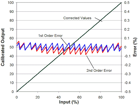 Figure 4. Calibrated output of a linear sensor input with first- and second-order correction |
 Figure 5. Calibrated output of a quadratic sensor input with first- and second-order correction |
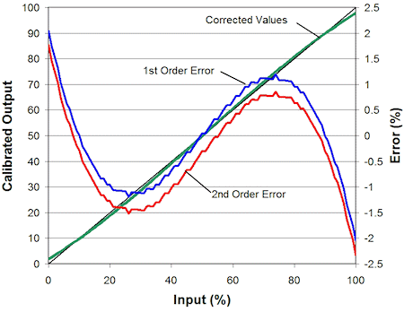 Figure 6. Calibrated output of a cubic sensor input with first- and second-order correction |
As expected, we obtain the best results when the order of correction matches the order of the input. Notice, however, that when second-order correction is applied to a linear sensor, the resulting error actually gets slightly worse, and test resources will be wasted taking unnecessary calibration data. Also notice that there is no significant difference in performance between first- and second-order correction when applied to a third-order sensor response.
The results in Figures 4, 5, and 6 are only for the first (and simplest) two methods. Unless direct observation rules some out, there are eight remaining methods to evaluate, with up to four additional variables, two of which are quadratic in nature. So, while making general observations by comparing sensor response to available correction algorithms can help rule out inefficient algorithms, selecting the best one from the remaining options is not trivial. This is where design support from the SSC manufacturer comes in. Without it, the designer must research and understand the details of each method, reproduce them in software, and run test cases for each method to determine which one is optimal.
Support Tools
Referring back to the SSC example in Figure 1, the SSC comes with hardware and software that allows a designer to select and evaluate the calibration methods quickly and easily. The hardware interfaces with a PC via USB and enables the designer to acquire and view data, and to program the appropriate calibration coefficients and set-up registers automatically. Software installed on the PC guides you through the process of data acquisition, recommending what measurements to make, and helping you to select the best calibration method based on your measurement results and system requirements.
Figure 7 is a screen capture of development support software for the SSC showing the data points necessary for a four-point calibration routine. After collecting input from the user about the input and temperature ranges, the software will guide you through a series of similar measurements for each of the calibration methods selected from Figure 2. The entire set is shown graphically in Figure 8, which is essentially a pictorial representation of Figure 2. Once all data have been collected, the software calculates the necessary coefficients for the selected algorithm and programs them into the SSC. The software has a test function that enables you to evaluate the calibration methods, compare them, and determine which one is best suited for the sensor and its application. For the production environment, a dynamic link library is available that will generate coefficients and register values for the selected algorithm from calibration points measured with automated test equipment. The production tester makes the required measurements, passes the results to this program, and then programs the returned values into the device under test.
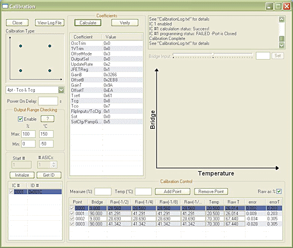 Figure 7. Screen capture of software aid for selecting and evaluating calibration methods |
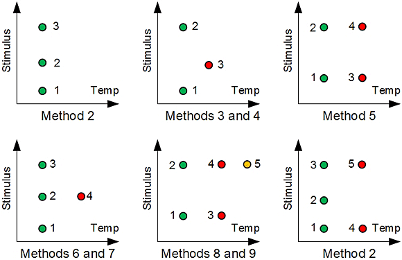 Figure 8. Sequence of measurements for obtaining correction algorithm coefficients |
Hardware and software support, such as described, is a tremendous benefit to the designer, facilitating rapid development of a sensor interface without requiring you to have intimate knowledge of the built-in algorithms or to recreate them in separate software to evaluate them for accuracy and to select the optimal solution. When selecting a sensor interface IC, the designer must look at datasheet parameters such as voltage and temperature ranges, ADC resolution, and noise levels. The level of expert knowledge and development support provided by the manufacturer is as important, if not more so, as the specifications. Choosing the wrong correction algorithm will diminish sensor system performance while increasing the development time, the resources used, the production cost, and your frustration level.
ABOUT THE AUTHOR
David Grice is a System Architect at ZMD America Inc., Pocatello, ID, providing engineering support for designers of custom ASICs and standard product ICs. He can be reached at 208-478-7200, [email protected].