
The noise characterization guidelines we present in this article are general in nature and based on recommended industry practices; users must apply their actual experiences and development efforts to optimize designs and processes for their testing techniques. The goal of the experiment we describe is to establish reliable estimates of the resolution of MEMS accelerometers.
Feature Description
Customers are often faced with the dilemma of selecting an appropriate accelerometer that is capable of providing the necessary precision for their application. Ultimately, the noise floor of the sensor determines the resolution, which is dependent on bandwidth. Therefore, it is very important to identify the inherent accuracy of the sensor and establish the accuracy of the ADC. To properly characterize the noise performance of these sensors it is critical to isolate an accelerometer from external vibrations. Characterizing accelerometer performance requires that noise due to external mechanical and electrical sources be separated from the noise intrinsic to the sensor.
Defining the Inherent Accuracy of Sensors
The sources of accelerometer noise can be broken down into the electronic noise from the circuitry that is converting the motion into a voltage signal and the mechanical noise from the sensor itself. There are several sources of electronic noise—Johnson noise, shot noise, flicker noise, and so forth—that are discussed in detail in many electronic and electrical engineering textbooks. The ASIC inside Kionix's accelerometer products has been designed to reduce these sources of noise as much as possible. The mechanical noise of the sensor comes from thermo-mechanical noise and environmental vibrational noise.
Thermo-mechanical noise (or Brownian noise) derives from the fact that MEMS accelerometers consist of small moving parts. These small parts are susceptible to the mechanical noise that results from molecular agitation. Fundamentally, the magnitude of the thermo-mechanical noise density (NDthermo-mech), which has units of g/√Hz, is given by Equation 1:
 | (1) |
where:
| kB | = | Boltzmann's constant (1.38 x 10⁻²³ J/K |
| ω | = | resonant frequency in Hz |
| m | = | mass in kg |
| Q | = | damping |
| T | = | temperature in K |
| g | = | acceleration |
In the absence of large environmental vibrations, thermo-mechanical noise is often one of the limiting noise components of MEMS accelerometers. As with the electronic noise of the ASIC, good sensor design practices reduce the thermo-mechanical noise.
Test Environment
Attention to the environment is important to obtain accurate noise measurements of a given accelerometer. Mechanical vibration noise sources operating nearby, such as compressors or other machinery, can cause inaccurate sensor noise readings. When characterizing the noise performance of a sensor at Kionix, the sensor under test is mounted on a large mass on an isolation table that floats on compressed air. The isolation table is placed in a room on the ground floor to minimize building vibrations. The room is temperature-controlled and quiet, with no heavy machinery operating nearby. Rapid fluctuations in temperature could cause variations in the output that are perceived as noise. If noise measurements are being performed in a temperature chamber, it is extremely important that fans, compressors, and solenoid valves remain off while the data are being collected. For electrical isolation, the sensor under test is typically powered using a battery rather than a DC power supply because the battery provides a clean DC voltage without coupling any 60 Hz noise into the system.
Analog Noise Measurements
For analog accelerometers, the output voltage measurements are made with an AC-coupled oscilloscope or an AC voltmeter. Readings are averaged to obtain the average RMS amplitude; this is the accelerometer RMS noise in volts. To determine the accelerometer RMS noise in g's, divide the RMS voltage by the sensitivity of the accelerometer.
Noise Density
To calculate an accelerometer's noise density (ND), you need to know the equivalent noise bandwidth, B, of your system. For a first-order simple RC low-pass filter (the most common filter type), B = 1.57ƒ–3dB Hz
For other filters, the noise bandwidth will have other values. For example, a Butterworth filter will give the following noise bandwidths:
B = 1.57ƒ–3dB Hz (1st order)
B = 1.11 ƒ–3dB Hz (2nd order)
B = 1.05 ƒ–3dB Hz (3rd order)
B = 1.025 ƒ–3dB Hz (4th order)
Once the noise bandwidth is known, Equation 2 is used to calculate the noise density parameter of an accelerometer from the measured RMS acceleration noise (an):
| (2) |
As an example, the noise density you might measure with a Kionix KXSS5-2050 accelerometer with a 50 Hz first-order low-pass filter would be:
The noise density is a useful parameter because it allows you to quickly calculate the accelerometer noise (and resolution) for different filter designs.
Digital Noise Measurements
While performing digital measurements, one should pay special attention to the Aliasing/Nyquist Theorem. Thus, sensors to be tested should be bandwidth-limited accordingly. The required sampling frequency in accordance with the Nyquist Theorem is the Nyquist frequency (fN) given by Equation 3:
| (3) |
where:
| ƒ–3dB | = | low-pass filter cutoff frequency |
To reconstruct the signal accurately, we recommend that the sampling rate be between five to ten times the low-pass filter cutoff frequency. Please also note that no dynamic tests were done in this experiment to characterize the ADC performance. The intentions of this experiment were purely to define the input-referred noise, otherwise known as code-transition noise. In an ideal ADC, the input analog voltage is increased and the ADC maintains a constant output code until a transition region is reached, at which point the ADC instantly jumps to the next code value and remains there until the next transition region is reached. In practice, an ADC has a certain amount of code transition noise and, therefore, a finite transition region width [1]. Input-referred noise is generally characterized by examining a histogram of a number of output samples while the input to the ADC is held at a constant DC value.
To measure the input-referred noise, the input to the ADC needs to be heavily decoupled by setting the low-pass filter frequency to 50 Hz or lower and then a large number of samples can be collected and plotted as a histogram (around one million conversions are more than adequate for a low-noise ADC). Because the noise is approximately Gaussian, the standard deviation of the histogram is the RMS noise (Figure 1).
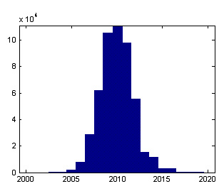 Figure 1. ADC output code |
As we can see in Figure 1, there is also some inherent differential nonlinearity (DNL) associated with this ADC but, for the most part, it is still approximately Gaussian. If there is significant DNL, but the results still follow a somewhat Gaussian distribution, then the standard deviation should be computed for several DC input voltage values and the results averaged. A code distribution that is significantly non-Gaussian could indicate a bad PC board layout, poor grounding techniques, or improper power supply decoupling.
Reducing Noise
The input-inferred noise could be reduced by placing a higher-order filter on the outputs or by reducing the bandwidth of the filter. Of course, one of the penalties for placing a higher-order filter on the outputs is an increase in the number of external components required on the printed circuit board. Likewise, one of the penalties for reducing the filter bandwidth is the increase in the startup/response time of the outputs. Depending on the application, this may result in the application having a sluggish response to motion, which can lead to a poor experience for the user.
Another technique that can be used to reduce noise is over-sampling and averaging. In most applications, digital data from the accelerometer are used in computations or in control functions. These data are obtained either directly from the accelerometer or after the analog data from the accelerometer have passed through an ADC. In either case, the system is acquiring accelerometer information at a particular sampling frequency. The optimal sampling rate will depend on the particular application. For example, a cell phone screen rotation application may have a sampling rate of 10 Hz while a hard-drive protection application may require a sampling rate of 1000 Hz.
Oversampling involves sampling a signal using a sampling frequency that is significantly higher than that of the Nyquist frequency. For example, the cell phone screen rotation application may be acquiring data at a 100 Hz sampling frequency. Every 10 samples are averaged together and that average value is reported at a 10 Hz frequency and used in the application to determine whether the screen has rotated. In this way, the noise in the acceleration signal is reduced. If multiple samples (N) are taken of the same quantity with a random noise signal, then averaging those samples reduces the noise by a factor of 1/√N.
References
1. IEEE Std. 1241-2000. IEEE Standard for Terminology and Test Methods for Analog-to-Digital Converters
ABOUT THE AUTHORS
Scott Miller is Vice President of Engineering for Kionix Inc., Ithaca, NY. Kenneth Foust is Director of Technical Support for Kionix and Izudin Cemer is an Applications Engineer at Kionix. The authors can be reached at 607-257-1080, [email protected].