
You all remember Ohm's law and the definition of electrical resistance as the ability of a circuit to resist the flow of electrical current. Although useful, Ohm's law applies to only one circuit element and assumes it to be an ideal resistor. Real-world circuit elements are more complex and exhibit resistive, capacitive, and inductive behavior that together define its impedance.
Impedance
Impedance differs from resistance in two significant aspects. First, it's an alternating current (AC) phenomenon, and second, it is usually specified at a particular frequency. If you measure impedance at a different frequency, you obtain a different impedance value. By measuring impedance across a number of frequencies, you can extract valuable data about an element. This is the basis of impedance spectroscopy, and it is the fundamental concept underlying many industrial, instrumentation, and automotive sensors.
The impedance of an electric element can consist of resistors, capacitors, or inductors—or more typically, a combination of these three units. You can model this effect using imaginary impedance values. Inductors have an impedance of jvL, and capacitors of 1 / jvC. In this case, j is the imaginary unit, and v is the angular frequency of the signal. The impedances of these components combine using complex number arithmetic. The imaginary component of an impedance is called reactance, and in general, Z = R + jX, where X is reactance and Z denotes impedance. When exposed to a signal of increasing frequency capacitive reactance, X C reduces, and inductive reactance X L increases, leading to changes in overall impedance as a function of frequency. The impedance of a pure resistor will not change with frequency.
How to Analyze Impedance
To examine the impedance of an element when swept at different frequencies, you usually have to examine the response signal in either the time or the frequency domain. Analog signal analysis techniques, such as AC-coupled bridges, were commonly used to examine the signal in the frequency domain, but the advent of high-performance A/D converters has led to data collection in the time domain with subsequent conversion to the frequency domain.
You can use a number of integral transforms to convert data into the frequency domain, with Fourier analysis being a common approach. This technique takes a time-series representation of a signal and applies an integral transform to map the representation into its frequency spectrum. You can use the technique to provide a mathematical description of the relationship between any two signals. In impedance analysis, the relationship between the excitation current (input to the element) and the voltage response (output from the element) is of interest. If a system is linear, the ratio of the Fourier transforms of the measured time-domain voltage and current is equal to the impedance, and it is expressed as a complex number. The real and imaginary components of the resulting complex number form a key piece of the subsequent data analysis:
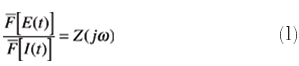 |
where:
E = system voltage
I = system current
t = time domain parameter
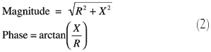
By converting the complex number to its polar form, you can determine both the magnitude of the response signal and the phase relative to the excitation signal at a particular frequency:
where:
R = the real part of the complex number
X = the imaginary component of the com- plex number
The magnitude calculated above is a representation of the complex impedance of the element at a particular frequency. In the case of a frequency sweep, you calculate this value at each frequency.
 |
Data Analysis
You commonly generate plots of impedance against frequency as part of your data analysis. A Nyquist plot is a parametric plot of the real and imaginary parts of the transfer function in the complex plane as the frequency is swept over a given range. If you plot the real part on the X axis and the imaginary part on the Y axis of a chart (the Y axis is negative), you obtain a representation of the impedance at each frequency. In other words, each point on the plot is the impedance at a particular frequency. You can calculate the impedance from the vector length |Z|, and the angle between this vector and the X axis is u. Figure 1 shows a typical Nyquist plot for a resistor and capacitor in parallel.
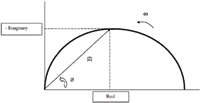 Figure 1. The Nyquist plot provides a representation of impedance at each frequency. |
Although often used, Nyquist plots don't provide information on frequency; it is therefore impossible to tell what frequency was used for a particular impedance. For this reason Nyquist plots are usually supplemented with other plots.
Another popular presentation is the Bode plot. In this case, the log of frequency is plotted on the X axis, and both the absolute value of the impedance |Z| and the phase shift are plotted on the Y axis. The Bode plot presents impedance and phase shift as a function of frequency. Usually, the Nyquist and Bode plots are used together to understand a sensor element's transfer function (see Figure 2).
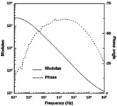 Figure 2. Bode plots let you examine both phase shift and impedance as a function of frequency. |
Impedance-Based Sensors
Under normal conditions, a sensor's impedance signature is based on its capacitive, inductive, and resistive combination. If a change in the sensor's environment causes any of these values to change, the sensor's impedance will change. By examining the sensor element over frequency, a new impedance profile will result as a consequence of this change.
A relatively simple technique for doing this is to compare a measured impedance profile with a predetermined profile. For example, take a metal-detection sensor using eddy currents as its operating principle. A high-frequency AC signal source is connected to a coil embedded in the sensor housing. The resulting electromagnetic field generated by the coil induces eddy currents in a conductive target. This in turn interacts with the sensor coil and changes its impedance.
Examining the impedance of the coil over frequency provides a number of benefits. For example, because the permeability of the material will affect the impedance of the coil, you can use empirical impedance signatures to draw conclusions about the type of metal the sensor is detecting. This process makes it possible for the sensor to detect metals of different permeability. You can also use permeability change to measure stress in metals because changing stress will change permeability, which in turn will change impedance.
Bode and Nyquist plots are useful in examining the frequency response of the sensor. Examining impedance over a number of frequencies provides a more accurate result than a single-point measurement because it helps average out noise. It also lets you identify the optimal operating point by examining the frequency response of the capacitive and inductive components under particular conditions.
Comparing measured-impedance with expected-impedance profiles can be applied to many different impedance-based sensor technologies, where resistive, capacitive, or inductive changes are provoked. Common applications include gas detection using a chemical sensor, moisture detection using capacitive-based sensors, metal coin or particle signature recognition in the gaming or food industries, and soil monitoring in the agricultural sector.
More Than Just a Sensor
Impedance analysis can involve more than simply comparing an impedance response to an expected profile. Impedance spectroscopy (IS) is also commonly used to characterize systems and to extract valuable information about them. For the purposes of this article, a system is broadly defined as an element or material in electrical contact with electrodes. This can be a solid-solid (in the case of many chemical sensors) or solid-liquid (when examining concentration of a species in a liquid) interface. You can use IS to obtain information about the element itself and the interface between the element and electrode.
IS takes advantage of the fact that a small voltage potential applied to the interface will polarize the interface. The manner in which the interface polarizes, combined with the rate at which it changes when the applied potential is reversed, characterizes the interface. This allows you to extract information about the system interface, such as adsorption/reaction rate constants, diffusion coefficients, and capacitance. And you can estimate information on the dielectric constant, conductivity, mobility of charge equilibrium, constituent concentrations, and bulk generation/recombination rates of the element (i.e., the sensor or substance under investigation).
To analyze data generated by the impedance sweep, you can use an equivalent circuit model of the system or element. The model combines resistors, capacitors, and inductors connected in such a way as to mimic the electrical behavior of the system. You look for a model whose impedance matches the measured impedance profile across frequency. Ideally, you choose the model components and interconnections to represent a particular electrochemical behavior, and the choice of components and interconnections is based on knowledge of the physical characteristics of the process. You can use an existing model from the literature, or you can empirically develop a new model.
When a model is developed empirically, you look for the best match between the empirical model and the measured data. The model components may not always correspond to physical characteristics of the process and can be constructed solely to give a best fit. You can build empirical models by successively adding and subtracting component impedances until you obtain the best fit. This is usually conducted on the basis of a nonlinear least squares (nlls) fitting algorithm. With the aid of a computer, the nlls algorithm takes initial estimates of the model parameters, successively changes each of the model parameters, and evaluates the resulting fit. The software progresses iteratively until the fit is considered acceptable.
Often, you can construct several different empirical models and have all of them provide the same impedance profile. You can also get a good least-squares fit but still have an incorrect model that is not representative of the physical system. And the nlls fit algorithm can ignore part of, or fail to converge on, the measured profile. This is because many algorithms attempt to optimize the fit over the entire spectrum but overlook poor fits at various points of the spectrum.
Treat the data analysis and equivalent-circuit modeling with caution and perform as much model validation as can be done. It is usually possible to build a good-fitting model by adding components, but this does not suggest it is representative of the system's electrochemical processes. In general, empirical models should have a minimum number of components, and, where possible, you should use physical models based on theoretical underpinnings of system processes.
 An Integrated Architecture for Impedance Measurement |
Corrosion Analysis
Corrosion analysis commonly uses IS to characterize a system. Corrosion of metals, such as aluminium and steel, is a significant safety concern in many industries, and can lead to premature failure if ignored. The ability to automatically monitor corrosion offers significant cost, safety, and reliability benefits and can help optimize preventive maintenance systems.
In addition to determining the degree of corrosion, you can predict metal fatigue by monitoring the rate of corrosion. As metal fatigues, it moves from elastic to inelastic behavior, and small cracks appear. These cracks are new but corrode relatively quickly, and the rate of crack propagation and subsequent corrosion indicates the level of fatigue.
Early identification of signs of corrosion, especially in hard to reach locations where visual inspection is impossible, helps to prevent or slow down the onset of serious corrosion. The same approach works for evaluating protective coatings under real-world conditions.
You can construct an equivalent electrical model of the corrosion process based on knowledge of the physical properties and the electrochemical processes that occur during corrosion. A common equivalent circuit for corrosion monitoring is a resistance Rs in series with a resistor (Rp) and capacitor (Cc).
In model A, the resistor Rs models the solution in which the metal resides, and the capacitor Cc models the protective coating or paint on the metal (see Figure 3). This represents the capacitance of the initial coating. After a period of time, water penetrates the coating and forms a new liquid/metal interface. As the metal corrodes, ion-conducting paths are formed through the protective coating between the solution and the metal. This is modeled by Rp in parallel with Cc. In addition, some models (model B) have an additional R and C combination in parallel connected in series with Rp to model delamination of the protective coating from the metal over time.
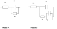 Figure 3. Equivalent circuit models are used to model the corrosion process. Model A depicts basic corrosion from an external source. Model B additionally models delaminating of the protective coating from the metal. |
The resistance or conductivity of the solution in which the metal resides is usually known or can be easily obtained, so Rs will be available. The value of Cc is also available because it can be calculated from the dielectric constant of the protective coating (usually provided by the manufacturer) and the area it covers. The technique then involves solving for Rp to determine the degree of corrosion. You usually achieve this with a curve-fitting algorithm to get a best fit to the measured impedance profile data. Bode plots are commonly used to examine the corrosion sensor's behavior in terms of its impedance and phase response over frequency.
IS is not limited to corrosion analysis, and can be used to characterize a range of electrochemical systems. For example, it can help optimize fuel-cell performance, predict battery health, examine the concentration of a species in a liquid to determine its quality, and characterize the electrochemical performance of a material.
Electronic Support Circuitry
Once the equivalent circuit model is validated, you have to design the electronic data acquisition system to perform the frequency sweep and capture the data. This is often a complex and time-consuming activity, requiring significant electronic skills to optimize the electronic-circuit designs.
You must design circuitry to generate the frequency sweep of a desired resolution over the range of interest. In many electrochemical systems, you have to avoid letting data collection interfere with the electrochemical process. This requires using small AC signals, and it's advisable that you do not introduce a DC potential difference across the system, which can induce further electrochemical activity.
The A/D converter must then acquire the system response to the excitation frequency. Some designs require two A/D converters to capture the excitation and response signals. This can be complex because simultaneous sampling of the A/D converters is required to allow the detection of phase changes between the signals.
In addition, the overall system must remain linear. In other words, the overall bandwidth of the system must be adequate, and signal sizes must be large enough to get good measurements—but not so large that they over-range the A/D converter or any other components and cause distortion. Because the element under test often has an unknown impedance range, some trial-and-error experimentation is often initially needed to optimize the system and ensure that it remains linear.
Once converted to the digital format, the response signal is usually presented to a computer for subsequent analysis. Newer approaches perform much of the analysis on the chip by extracting the real and imaginary components of the response signal before subsequent processing on a computer. This relieves the computer of performing significant arithmetic functions and improves data collection because the analog signal processing circuitry is optimized to operate with the other functional blocks. Remember that although computers can easily provide results extending to four or more digits, unless the measurement of the analog signals is valid and attention is given to ensuring that the overall system remains linear, the result will contain errors. Careful system design and validation to obtain valid measurement are critical to the accuracy of the result.
James Caffrey, MEng, can be reached at the Precision Signal Processing Group, Analog Devices, Inc., Limerick, Ireland; 011-353-612-29011, [email protected], www.analog.com.