

Part 1 of this article in the August 1999 issue of Sensors examined component vibration test theory, which suggested the exploitation of component dynamics and modes of vibration for defect detection. Concepts of dynamic forcing functions and component frequency response functions (FRFs) were presented as a basis for constructing a test strategy for component assembly line acceptance tests. The equations and figures in Part 2 are numbered consecutively from those in Part 1.
In the time it takes the average reader to read this article, more than a million bearings will have been manufactured for inclusion in more than 2000 components that will be integrated by tier-one suppliers into more than 1200 different products.
Consider a manufacturer of alternators as a tier-one component supplier to an automaker. A bearing manufacturer produces ball bearings at tier two or tier three and incorporates them into a bearing assembly to sell to the alternator manufacturer. The bearing is assembled on a shaft, the primary structural element of the rotor assembly, which is then assembled with housing, including field windings and various electrical parts to complete the alternator component. These components will be produced at a rate from several hundred to two thousand per day. The tier-one supplier understands that life or death as a business depends on delivering alternators free of defects.
The whole process is completed with the arrival of an automobile at the end of the assembly line where a QC inspector simply starts the engine and listens to it idle. This can be a most dramatic moment for a few tier-three steel balls spinning in the alternator-bearing race--and the worst nightmare for the tier-one alternator supplier! At this point, slight imperfections in the balls could introduce vibration that manifests itself as noise at a level that causes the inspector to reject the entire vehicle on the spot.
Actually, alternator suppliers avoid this scenario, rejecting defective units on the line using fast-acquisition vibration measurements. Some automakers require their suppliers to perform assembly line tests of this type. The test station is typically capable of processing a unit about every 15 s, including run-up, electrical functional checks, and dynamic defect detection.
 |
| SigQC performs early detection of component defects to avoid rejection on the final product assembly line. |
Preprocessing Vibration Signals
At this point it is appropriate to introduce some basic concepts of acquiring and preprocessing dynamic sensor signals because signal processing is an important part of the defect detection process.
Rapidly fluctuating transducer signals proportional to desired physical measurements are input to a high-speed computer-controlled data acquisition system. For example, signals representing displacement, x(t), and force, f(t), are simultaneously sampled into a computer, producing sets of discrete synchronized displacement and force values separated in time by some small time increment, Δt. The assembly line pass-fail process is often based directly on these time domain data. However, much of our discussion will emphasize the use of data that have been preprocessed to produce various forms of frequency domain data.
The basic path to the frequency domain is via the fast Fourier transform (FFT). FFTs performed on the sampled displacement x(t) and force f(t) time functions produce frequency domain data sets characterized by amplitudes at discrete frequencies. The French physicist and mathematician Jean Baptiste Fourier (1768–1830) proved that any periodic function of time can be represented as the sum of an infinite series of cosine waves and sine waves. The terms in the summation will have suitable amplitudes and frequencies that are integer multiples of the fundamental frequency that has a single cycle in the time period. The FFT processes data over a finite time period, but treats the data mathematically as though it were just one period of a cyclical set of data extending over all time, from minus infinity to plus infinity. That is, the set of data acquired over some time period, T, is treated as though it repeats itself indefinitely, allowing the application of the Fourier series. The cosine and sine amplitudes of the Fourier series are stored as real and imaginary numbers, respectively. Thus, the FFT produces a spectrum of mathematically complex amplitudes. The discrete frequencies are separated by some fixed increment, Δn (frequency increment in Hz).
In practice, an FFT is performed on short bursts of data having a time period, T, of perhaps 0.1–5.0 s duration, depending on the available data storage capacity and desired sampling parameters. As a consequence of discrete signal sampling theory, the frequency domain data resolution, Δν, of an FFT performed on data of duration T is:
![]()
Equation (15) implies that the first frequency line of the FFT spectrum (lowest non-zero frequency) corresponds to that of a sine wave completing one cycle in the time period T. All other discrete frequencies in the spectrum are integer multiples of that first frequency. The highest frequency, νmax, in an FFT spectrum having M frequency values ("frequency lines") would be:
![]()
The frequency increment for our purposes must be small enough to provide adequate definition of peaks in the frequency domain data. The frequency range of interest is ensured by acquiring the time domain data, x(t) and f(t), at a sufficiently high sample rate, SR. Shannon's sampling theorem states that the maximum available FFT frequency,νmax, will be one-half of the sampling rate, SR:
![]()
SR, of course, corresponds to acquiring one data point in the time domain with each increment of time, Δt, that passes:
![]()
The computer array size (number of data points), p, required to store one time function sampled at a rate, SR, over the time period, T, would be:
![]()
Finally, it can be shown using the above equations that the number of frequency lines, M, in an FFT spectrum is one-half of the number of data points, p, in the time domain for a given time period, T:
![]()
It is clear that understanding the relevant frequency range of component vibration phenomena, and then understanding the corresponding sampling and data storage requirements, is crucial to a successful test plan.
Inherent Signal Processing Errors
Once a continuous and rapidly fluctuating signal is captured in a computer, two types of error are guaranteed:
* Truncation error
* Digitizing, or sampling, error
Despite the ever-increasing megabytes of RAM and gigabytes of disk space, a computer is finite. A time series data set is ultimately stored in a finite amount of memory. A true sine wave, by mathematical definition, extends from minus infinity to plus infinity in time. A sine function stored in computer memory is not really a sine function because it has been truncated to fit into the available computer data array space. The effect of this truncation can be analyzed mathematically by carrying out the Fourier transform integral of a displacement sine wave function, x(t), multiplied by a box function, B(t). The box function is described as having a value of zero from minus infinity in time up to zero time, having a value of 1.0 from zero to the end of the time period, T, then continuing out to plus infinity in time with a value of zero. The product, B(t) * (t) exactly describes a truncated sine function:
![]()
Using the frequency domain convolution theorem, the result of the Equation (21) integral can be visualized quite easily:
![]()
where:
B(ω) * X(ω) the convolution of the Fourier transform of the box function with the Fourier transform of the original true sine wave
Instead of obtaining the true Fourier spectrum of a sine wave, X(ω) (which would manifest as a single non-zero value at a single discrete frequency), a distorted spectrum is revealed, Xtrunc(ω), having a host of additional frequencies spilling out into the neighborhood of the original frequency.
Fortunately, the amplitudes of these extraneous frequencies decrease exponentially as the frequencies move out away from the true frequency. This type of error is reduced by the use of special window functions as part of the normal signal processing. The end user need only be aware of the problem to ensure that the data acquisition and processing system used has addressed the truncation issue.
The sampling error problem is conceptually self-evident. By sampling a signal at intervals of Δt it is clear that lots of data have been skipped over. The discrete data points lifted from the signal are simply not the same thing as the original complete continuous function. This discretizing of the data can lead to enormous errors and misrepresentation in the frequency domain. Under certain conditions high frequencies will masquerade as low frequencies. The high frequencies are said to take on lower frequency aliases. The responsible data acquisition vendors have this problem well under control, and the end user should make sure that proper anti-aliasing features are part of the system [1,2].
FFT Scaling
The FFT has been scaled in various ways. Two common scaling practices are the sine wave peak amplitude scaling and the sine wave root-mean-square (rms) scaling. The sine peak amplitude scaling provides the peak value of a phase-shifted sine wave for each discrete frequency of the FFT spectrum.
The rms value of a sine wave is ~0.707 3 the peak value. The attraction of the rms scaling is that it is consistent with the statistical analysis and probability estimates used in the evaluation of product quality and success of defect detection strategies. The rms value at a particular frequency is essentially the same as the standard deviation for the corresponding sine wave as computed over the time period, T.
Consider filtering out a pure sine wave (having some phase) from a signal. Now, list all of the numbers constituting the signal value at each increment of time, spanning the complete time period, and compute the standard deviation for that set of numbers. The standard deviation will be quite close to the rms value. If you consider each of M phase-shifted sine waves in the spectrum to be statistically independent and to have standard deviations, σi, then the total statistical variance, VT, over the spectrum is:
![]()
A common form of frequency domain data is the power spectrum, or rms-squared spectrum. When scaled as rms, the conjugate FFT product directly produces a power spectrum. The conjugate product is used in view of the FFT complex amplitudes. The displacement power spectrum, SXX(ω), would be computed as:
![]()
where:
X*(ω) = the complex conjugate of X(ν)
The total power, STXX or X2Tot, over the complete spectrum would be:
![]()
Notice that this result is essentially the same calculation as Equation (23). This also means that the overall rms value of the signal over the time period, T, and including all frequencies, is just the square root of Equation (25):
![]()
The rms value computed directly in the time domain over the time period, T, would be:
![]()
We are assured by Parseval's theorem that the rms value for the frequency domain, Equation (26), should match the rms value for the time domain, Equation (27).
In practice, engineers like to average the power spectra, SXX, over 20 or more ensembles for better accuracy in the estimate of a component's stationary vibration characteristics:
![]()
The time required to acquire an adequate number of data sets (total time, n T) could conflict with assembly-line production rate requirements. It is necessary to understand the tradeoff between frequency resolution (which controls the time period, T), array size, frequency range, and ensemble averaging to develop a compatible set of test parameters. At some point it may be necessary to weigh product quality against production rates.
Data Signatures for Good Units and Defective Units
The type of frequency domain data useful in our process is suggested by the FRF, hjk(ω), developed in [3] for the dynamic force and resulting vibration response between any two points k (point of applied force) and j (point of measured response vibration):
![]()
In [3] we demonstrated that the response motion at any point can be thought of as a superposition of the individual responses of N vibrating mode shapes. That modal superposition is indicated by the summation in Equation (29). Each mode has a characteristic amplified response in the neighborhood of its resonance frequency, vr. Notice the effect on hjk(ω) as bβr (βr = vω/vωr) approaches a value of 1.0 in the denominator of Equation (29). The level of vibration for each mode at its resonance frequency depends on the mode coefficient values, Ψjr and Ψkr, at points j and k, as well as the modal damping ratio, ζr, and modal mass,
mr, for each of the mode shapes, numbered r = 1, 2, 3, . . . N. Thus, all of the vibrating modes taken together result in a physically measurable ratio of the response displacement, Xj(ω), to the applied force, Fk(ω):
![]()
The actual FRF computation forms the
ratio of averaged cross-power spectra, SXF(vω),
and the averaged autopower spectra, SFF(ω):
![]()
where the averaged cross-power is the average of n sequential complex conjugate products of displacement and force:
![]()
And the autopower of force is computed as previously shown in Equation (28) for displacement.
A matrix of FRFs, [ H ], characterizes the entire structure in terms of response motion at every point on the structure due to forces applied at any point or combination of points on the structure. The [ H ] matrix is intrinsic to a component such as an alternator, and for good units is defined once and for all time.
 |
| Figure 5. FRFs can be used as frequency domain data signatures for good and defective units. The FRFs shown here were generated analytically using Equation (29). Modal parameters were adjusted for two modes in order to create the defective signature. |
One or more FRFs selected from the [ H ] matrix could be used as the basis for detecting defects in a component as suggested by Figure 5. Two FRFs have been generated analytically, using Equation (29). One FRF representing a good unit used as a baseline is plotted together with an FRF representing a unit having a defect that affects the vibration response of two modes. Mode coefficient values, damping, and resonance frequencies were altered for these two modes.
Notice in Figure 5 that the defect caused deviations in the FRF over an extended frequency range in the neighborhood of each of the two affected modes. This is a consequence of altering each of the two single-degree-of-freedom (SDOF) modal FRFs over their entire frequency range [3]. FRFs thus provide distinct signatures in the frequency domain.
Let's now assume, for the sake of our example, that the Figure 5 FRFs had been processed from a measured forcing function, f(t), and displacement response function, x(t). Next assume that a hammer impact was used to apply force to the unit under test. The hammerhead is equipped with a force transducer, and a laser vibrometer measures displacement. Further assume that the FRFs of Figure 5 are computed using Equation (29).
 |
| Figure 6. These vibrational signatures represent displacement response functions resulting from hammer impacts on a good unit (A) and a defective unit (B). Each unit yields a unique time domain signature. |
Notice that we could have used the displacement function, x(t), directly as a time domain signature. The time domain signatures for good and bad units would appear as shown in Figure 6.
The fact that a test unit is always characterized by a matrix of FRFs, [ H ], whether FRFs have actually been measured or not, guarantees that a specific time signature will be produced under a particular impact force, f(t). The Fourier transform of the displacement transient measured at point j due to an impact at point k must be the product of the FRF and the Fourier transform of the impact force:
![]()
And the displacement time function, x(t), is just the inverse Fourier transform:
![]()
Or, in signal processing terminology, the displacement time function is the inverse FFT (IFFT) of the displacement FFT:
![]()
This emphasizes the specific causal relationship between an input forcing function and the response motion, and shows that either of two displacement signatures is available from an impact test: the FFT spectrum signature of Equation (33) or the time signature of Equation (35).
When sufficient time is available at the test station to perform multiple hits, the averaged displacement autopower spectrum would in many cases provide a more consistent signature than a single FFT spectrum.
Signatures for Operating Products
Now consider a product such as an electric motor positioned in the test station on the assembly line. For this example we will assume that provision has been made to operate the motor in the test station at an rpm corresponding to normal use. The operational unit is now providing its own forcing function, f(t). In fact, considering the spatial distribution of the magnetic force field between the rotor coils and the poles of the magnet, we recognize that a set of pulsating forces is present. But we expect that all good units will generate the same set of forces. And reflecting on the role of the [ H ] matrix in the vibration process for this structure, we understand that these pulsating forces must produce a specific causal set of displacement responses around the alternator case in accordance with the system simultaneous equations in matrix form:
![]()
The numbered rows of the column matrices, {X(ω)} and {F(vω)}, correspond to numbered degrees-of-freedom throughout the motor structure. Most of the elements in the {F(vω)} column would have values of zero, while elements corresponding to magnet pole and rotor coil locations would have force Fourier transform functions representing the pulsating forces.
The purpose of presenting Equation (36) is not to imply that we will measure the [ H ] matrix and the pulsating forces and compute displacement motions, but rather to establish a conceptual model for the vibration process. It follows that a signature useful for defect detection would be the averaged displacement autopower spectrum. The motor would have to run sufficiently long to acquire the required number of data sets for the averaging indicated in Equation (28).
Operational Time-Dependent Signatures
It is not uncommon to encounter operational units that perform a particular duty cycle, such as automobile sun roofs and power window mechanisms. The duty cycle sometimes proceeds through stages in which a new set of forces develops for each stage. Even when the motor excitation forces remain fairly stationary, the structure itself may be changing, altering mode shapes and resonance frequencies.
The averaged autopower spectrum works well in such cases. Averaged power spectra are continuously processed and displayed as a function of time in a 3D waterfall format, 3D carpet plot, or any preferred 3D graphics display. This provides a 3D signature that is constant for good units and produces deviations for defective units.
Sometimes a single overall time domain signature is used, in which the time-averaged rms value of a signal is displayed as a running average. This provides limited information as compared to a running average of the autopower spectrum.
Order Analysis Signatures
Assembly line tests for motors sometimes require a run-up operation in which data are continuously sampled while the motor rpm is continuously increased from zero to some maximum. This results in continuously increasing frequencies associated with an increase in the pulse rate of the magnetic forces. Furthermore, the Fourier transform of a pulsating force reveals an extended harmonic series of frequencies. The fundamental frequency is accompanied by a large number of harmonic frequencies, all integer multiples of the fundamental frequency. Thus, for the run-up operation, we have a fixed pattern of frequencies that are continuously increasing in frequency values.
Again, the 3D graphics display of autopower spectra provides a signature for identifying either good or defective units. Sometimes called a speed map, an isometric view of the data surface reveals two kinds of effects: ridges of peaks stationary in frequency and ridges of peaks shifting in frequency, following a path in time consistent with the changing motor rpm. The fixed ridges correspond to resonant response at the fixed resonance frequencies of the structure.
Another popular 3D graphics signature that is unique to run-up operations results from a signal processing procedure known as order analysis. A tachometer provides a continuing measure of rpm throughout the duration of the run-up test. Using these data as a reference, the frequencies corresponding to the harmonic series are computed. The order analysis uses only those autopower spectrum amplitudes that correspond to the fundamental and harmonic frequencies, or orders. The graphics display X-axis is scaled by order numbers (1, 2, 3, . . .); the Y-axis is scaled for autopower amplitude; and the Z-axis is scaled for time. The ridges of peaks corresponding to orders actually remain stationary (fixed X-axis values) on the 3D plot.
 |
| Screen 1. Additional mathematical and logical processing may be performed on data that have been preprocessed by front-end analyzers or plug-in cards. A graphical user interface facilitates the programming. |
Nonlinear Frequency Domain Signatures
The world of sound and acoustics has a long tradition of processing frequency data into 1/3 octave bands rather than the linearly spaced frequencies of the FFT. That tradition arose partly as a result of the early limitations of technology and partly out of a rough correspondence between subjective human hearing characteristics and 1/3 octave bandwidths. For whatever reason, 1/3 octave analysis is now quite popular in vibration applications. Present-day signal processors provide a range of nonlinear frequency options: 1, 1/3, 1/6, 1/12, and 1/24 octave.
When processing averaged autopower spectra, for example, the nonlinear frequency analysis actually achieves significant improvement in efficiency as compared to the FFT. The FRF frequency bandwidths of SDOF structural modes typically get broader as frequency increases. This means that less frequency resolution is required as frequency increases across the spectrum. In fact, the changing structural bandwidth matches a 1/n octave spacing of analysis frequencies.
The nonlinear frequency spacing is described by:
![]()
where:
n0 = a selected initial frequency
nn (n = 1, 2, 3 . . .) = the 1/n octave center frequencies
The keys on a piano are spaced at 1/12 octave frequency intervals, beginning with note "A," having the frequency, ν0, equal to 27.5 Hz. The Acoustical Society of America and European standards organizations publish a standard set of center frequencies that is embraced as a worldwide industry standard.
Another approach to the frequency domain is to perform digital filtering over selected bandwidths.
 |
| Screen 2. A target function is generated, setting the goal for good product performance (black acceleration trace). The red tolerance band establishes upper and lower limits of acceptance. Limit statistics such as standard deviations may be computed automatically. |
 |
| Screen 3. Data from a unit having a known failure mode is compared to the target function (black curve) and the red tolerance band. Simultaneous out-of-tolerance conditions within a specific set of frequency bands can fingerprint a particular failure mode. |
Sensors
Displacement has been used throughout this article to represent the response motion of vibrating structures. And the laser vibrometer is often the sensor of choice for this measurement. The purpose here was to maintain a consistent thought process, which had its beginning in the solution of the second order differential equation for a SDOF system [3].
But other sensors and other choices for representing motion could have been cited. Microphone sound data and dynamic pressure measurements are frequently used as well [4]. Accelerometers are probably the most popular vibration sensors due to their freedom of placement, wide frequency range, and wide dynamic amplitude range. In addition, data can easily be converted among displacement, velocity, and acceleration information as part of the signal processing process. This is particularly true in the frequency domain where the FFTs for these three parameters are related through simple algebraic formulas [5].
The laser vibrometer does have one distinct advantage for assembly line test stations. A vibrometer designed with a small optical head at the end of a flexible fiber-optic cable is particularly attractive in applications where deflections are not overly small. The vibrometer can be fixed in place, whereas an accelerometer must physically engage each unit coming down the assembly line. The engagement mechanism tends to require some level of design sophistication, and the coupling of the accelerometer to the unit under test is critical.
Defect Detection Software Implementation
The SigQC software system from Signalysis, Inc., has been developed to automate dynamic defect detection on the assembly line. The software has been designed to support four phases of activity encountered in the total test effort:
- Develop the basic test method
- Develop an acceptance test strategy
- Perform assembly line defect detection
- Perform postproduction activity
The product vibration and/or acoustic characteristics are revealed during the first phase of activity. A theory-based strategy would lead to extensive testing and analysis, including modal testing and perhaps finite element modeling. If the phenomenological approach is followed, the only area to receive attention will be the identification of any type of vibration phenomenon associated with defective units. In either approach, product characteristics are viewed using a variety of measurements and signal processing conditions. Ultimately, measurements and signal processing parameters that provide unique signatures for good and bad units are identified.
During the first phase, the test station has been configured and is in operation either on the assembly line or in an R&D environment. SigQC has been integrated with a number of different data acquisition systems varying in capabilities and cost from plug-in boards to top-of-the-line multifunctional real-time analyzers. Hardware setup conditions are accomplished from within the SigQC software. In addition to the signal processing performed in the front-end analyzer or plug-in card, SigQC provides graphics programmability for additional mathematical and logical postprocessing (see Screen 1).
SigQC activity is coordinated with assembly line action through automated interfacing to programmable logic controllers (PLCs). Communication is implemented through digital I/O (contact closures) and RS-232 serial communications. The logic between SigQC and PLC is established using on-screen graphics programming involving points and clicks and dialog field entries.
By the end of Phase 1 activity, large samples of data such as time transients, autopower spectra, or order analysis spectra have been collected from an adequate statistical sample of production units. An in-depth effort would separate a statistically large collection of units into groups: good units group, failure mode 1 group, failure mode 2 group, failure mode 3 group, etc. A minimal effort would follow the strategy of collecting a master data pool from which good units would later be identified based on a statistical matching of autopower or other signatures.
Acceptance Test Strategy
The primary goal of the Phase 2 activity is to develop pass/fail criteria for one or more acceptance tests. Different failure modes may require different test conditions. One motor failure mode might show up at low rpm during a run-up acceptance test, while another might show up in a nonoperating acceptance test using an FRF measurement. SigQC can automate a rapid sequence of tests. For each, several separate test cases may be applied, each enforcing a unique set of pass/fail criteria.
Working with the "target data pool," the data acquired from a large statistical sample of good units, a target function is generated against which measurements of production line units will be judged. For example, a target function could be established from the average of all autopower spectra in the target data pool. A tolerance band is then specified to establish the upper and lower limits of deviation permitted for acceptance of production line units.
Additional spectral fingerprinting is established by identifying frequency bands, within which special additional acceptance criteria are imposed. For example, it might be required that a specified number or percentage of data points must exceed a limit for rejection. Or some logical combination of conditions may be specified for a group of bands. A particular failure mode might be identified with out-of-tolerance conditions appearing simultaneously in a specific group of bands. These special rejection criteria are often developed through a review of data obtained from statistical samples of units with known defects. Some of the on-screen activity in establishing tolerance bands, frequency bands, and special rejection criteria are shown in Screen 2 . Screen 3 illustrates the review of data from a bad unit, comparing its spectrum to the target function and the tolerance band.
Assembly Line Operation
The sequence of activity at Phase 3, the assembly line test station, is programmed within SigQC using a flow chart graphical user interface. A library of test station actions is represented by icons available on an on-screen tool bar. The sequence of actions is implemented with drags, drops, and line connections to specify the order. Actions requiring coordination with the test station would have previously been accounted for during the PLC programming phase.
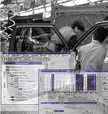
A database of acceptance tests with complete description of products, test setups, and pass/fail specifications is available for automatic access. An early action at the test station would be the identification of a unit just arriving at the station. A bar code scanner or keyboard entry would provide the computer with the information needed for automatic selection and initiation of the acceptance test. Upon test completion, SigQC signals the PLC with a pass/fail indication leading to automatic disposition of the test unit. Screen 4 indicates on-screen activity during assembly line testing. The icons in the flow chart are highlighted in sequence as the test station action proceeds. The data for the unit under test are rapidly displayed in a separate window. The data window border changes to red upon detection of a defective unit.
As production runs accumulate, reliability engineers and product managers engage in an offline review of product performance. SigQC provides historical database reporting and supports analysis for production control, including Pareto charts for assessment of specific failure modes.
We anticipate that this type of defect detection will find increased use in manufacturing plants as companies recognize the potential for exploiting the dynamics that characterize their products.
References
1. Michael Cerna and Mendy Ouzillou. July 1999. "Understanding Frequency Domain Measurements," Sensors, Vol. 16, No. 7:40-48.
2. John C. Cole. July 1999. "Acceleration Data Acquisition Using a D–S Converter," Sensors, Vol. 16, No. 7:55-60.
3. Neil Coleman and Robert E. Coleman. Aug. 1999. "Dynamic Defect Detection, Part 1: Theory of Vibrational Analysis," Sensors, Vol. 16, No. 8:14-24.
4. Bernhard Konrad and Martin Ashauer. July 1999. "Demystifying Piezoresistive Pressure Sensors," Sensors, Vol. 16, No. 7:12-25.
5. Jon Wilson. Feb. 1999. "A Practical Approach to Vibration Detection and Measurement, Part 1: Physical Principles and Detection Techniques," Sensors, Vol. 16, No. 2:12-27. March 1999. "Part 2: Dynamic and Environmental Effects on Performance," Sensors, Vol. 16, No. 3:52-60. April 1999. "Part 3: Installation, Recalibration, and Application," Sensors, Vol. 16, No. 4:46-56.
 |
| Screen 4. The test station action sequence is programmed in SigQC using a flow chart graphical user interface. Tool bar icons drag and drop and are connected for a specified order. Test unit data are displayed during assembly line testing. The data window border turns red for defective units. |