
Major bridges are designed to accommodate specific levels of traffic and wind loading, as well as to withstand deterioration over time. But it's not unusual for them to experience levels greater than those initially anticipated. As a result of these forces and thermal action, the large structures often move anywhere from a few decimeters to nearly a meter. While engineers use theoretical models to design the structures, they rarely compare the models with actual movement measurements. To factor in these real-world conditions, engineers are turning to a new application of an established technology.
Global Positioning Systems
GPS is a U.S. owned-and-operated satellite-based positioning system. The 28 satellites, orbiting Earth at an altitude of 20,000 km, transmit binary code modulated on carrier waves.
The conventional way of measuring ranges with known coordinates is to measure the time of flight of the timing codes. By knowing the time required for the signal to reach the GPS receiver from the satellite, you can calculate the range, and therefore calculate the coordinate of the GPS receiver based on simultaneous ranges from a number of satellites. This identifies a position accurate to within ~10 m.
Kinematic GPS
In addition to the timing code, survey-grade GPS receivers use the carrier signal to determine ranges. The carrier has a resolution of ~1 mm and a resulting 3D positional precision of ~1 cm.
Carrier phase positioning requires a reference GPS receiver to which the user's GPS receiver is coordinated. A variety of processing methods are used in this approach; one is kinematic GPS. Using this method, the roving receivers, whose coordinates are unknown, are positioned relative to reference receivers with known coordinates. Data processing can be carried out on the fly (OTF) in real time.
Kinematic GPS is ideal for monitoring large structures because it generates 3D coordinates at a typical rate of 10 Hz, producing 3D movement data for specific locations on the structure. In addition, the resulting movement measurements are in absolute terms (i.e., the coordinates can be repeated), and the GPS equipment requires minimal setup and calibration. Other devices, such as accelerometers and strain gauges, take longer to install and, at best, result in relative displacement data (i.e., the coordinates may not be repeatable in future trials).
The GPS-based system provides 3D coordinates with corresponding time, making it possible to derive the frequency of structural movements. Typically, the first natural frequency of long suspension bridges is 0.1 Hz; second- and third-order frequencies have been detected as well. You can analyze deflections in real time and compare them with the limitations of the bridge, and also analyze the frequencies of the movements and compare them with predicted values. GPS-derived data can be used to validate predictive models of the structure, and you can use the constant comparison of the models with the real movements to analyze structural health.
Putting GPS to the Test
From February 8–10, 2005, staff from the University of Nottingham's Institute of Engineering Surveying and Space Geodesy (IESSG) and from Brunel University's (West London) School of Engineering and Design investigated the use of GPS to establish the magnitude and frequencies of a bridge's deflections. The field research was conducted on the Forth Road Bridge, near Edinburgh, Scotland. The bridge has an overall length of 2.5 km and a main span length of 1,005 m. Traffic over the bridge has steadily increased from 4 million vehicles in 1964 to more than 23 million in 2002. In addition, the heaviest commercial vehicles weighed 24 tons in 1964; the current limit is 44 tons.
The project staff conducted trials at seven GPS-receiver locations on the bridge during a 46 hr. period. The bridge's GPS receivers were coordinated relative to two reference receivers located adjacent to the bridge, on the southern end viewing platform. The GPS receivers on the bridge were located on the east side mid span, ¼ span, ¾ span, and ⅜ span, as well as on the west side mid span and the top of the two southern towers. The receivers gathered data at a rate of 10 Hz. In addition, data from nearby Ordnance Survey's Active Station Network were downloaded at a rate of 1 Hz for future processing.
This article illustrates the kinematic GPS technique but analyzes only a small portion of the vast amount of data gathered during the trials. However, this subset of data demonstrates the accuracy and repeatability of the procedure.
During the trials, the data were processed after the event. Real-time processing is possible, but establishing real-time communications was beyond the scope of the feasibility trial.
Implementation
The Forth Estuary Transport Authority (FETA) fabricated clamps to attach the GPS choke ring antennas to the bridge's handrail in such a way as not to endanger passing pedestrians or cyclists (Figure 1).
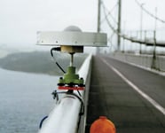 Figure 1. During the trials, the staff used clamps to attach the GPS choke ring antennas to the bridge's handrail |
The GPS data were recorded on internal data cards in the GPS receivers and simultaneously downloaded approximately every 12 hr. Due to the high resolution of the GPS carrier-phase data used, the precision of the 3D results is at the millimeter level. OTF kinematic processing produced data files that consisted of World Geodetic System 1984 (WGS84)–compliant coordinates, at intervals of 0.1 s. The resulting 3D coordinates were transformed into bridge coordinates. Postprocessed OTF data generated approximately 11 million coordinates. This is a huge amount of data, so initial analysis focused on specific occurrences.
In addition, an Omni Instrument weather station was located adjacent to the west-side GPS receiver, gathering air temperature, pressure, relative humidity, and wind speed and direction readings every 15 s.
Results
Figure 2 illustrates the relationship between the air temperature and height deflections at site F (the western side of the bridge). Changes in temperature alter the length of the cables and hence the vertical position of the bridge's deck. This shows the relationship over a temperature change of ~5.5°C. Over a one-year period, the air temperature at this location can change by 30°C, hence a larger vertical change can be expected. .
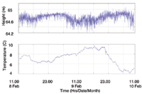 Figure 2. The relationship between air temperature and height of the western side of the bridge s deck |
The staff then applied spectral analysis to the data. Figure 3 illustrates the results from site F. Note the three distinctive spikes in the results (upper trace). The main spike corresponds to 0.1055 Hz and is the first natural frequency of the bridge. The other two spikes possibly correspond to other natural frequencies of the bridge. .
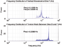 Figure 3. The trial data show the natural frequencies and torsional frequency of the bridge |
During the second night, two 44-ton trucks were used as a control loading of the bridge. These trials were carried out a couple of hours after the high winds subsided slightly, and during these trials, the bridge was closed to other traffic. The trucks started the trials at the north end of the bridge and proceeded as follows:
- 1. One truck ran from north to south.
- 2. One truck ran from the south end of the bridge to mid span on the west side and stopped; then the other truck moved north to south.
- 3. One truck moved from north to south and stopped at mid span; the other moved south to north.
- 4. One truck moved from south to north, and then both moved side by side north to south.
The trucks traveled at 20 mph. Figure 4 shows the changes in the bridge's height throughout the trials. The bridge deflected by as much as 400 mm due to the combined 88-ton loading. .
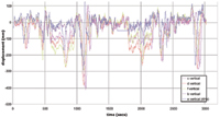 Figure 4. The height deflections of the bridge during the truck trials |
Figure 5 illustrates the final maneuver, whereby the two trucks traveled from north to south, side by side. Keep in mind that vehicles travel on the left side of the road in the U.K. and that the bridge is orientated north to south. The graph also shows the physical location of the trucks at any time (e.g., north tower, mid span, and south tower). .
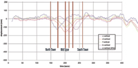 Figure 5. The data show height deflections of the bridge occurring during the period when the two 44 ton trucks passed side by side over the bridge |
Three main phenomena are evident in Figure 4. First, the deflections are offset by each other in the same way they were for Figure 3.
Second, the GPS receivers located at sites D (the eastern side) and F (mid span) deflect by different magnitudes, even though they start off at the same height. This is due to the torsional movement of the bridge. The trucks, traveling in the left lane from north to south, were traveling on the east side of the bridge. Hence the eastern side deflects more than the western side (site F).
Third, note that the bridge consists of three separate spans, each connected by a cable that passes over the top of the towers. As the trucks pass over the northern span, the load pushes this smaller span down, which in turn pulls down the hanger cables and the suspension cable to which they are attached. This results in the suspension cable pulling up on the main span. The trucks pass onto the main span, and as they pass to the south side span, upward movement of the main span (described earlier) is observed. In addition, the sinusoidal nature of the bridge's movement is visual in this data.
Next: GPS and FEM
Early bridge deflection monitoring trials showed that carrier-phase GPS can detect sub-centimeter movements and calculate the frequencies of these movements. Currently, the staff is carrying out this work with dual-frequency surveying-grade code- and carrier-phase GPS receivers. The trials at Scotland's Forth Road Bridge have shown that it is feasible to use GPS to measure the magnitude and frequencies of the bridge's deflections in 3D. This is possible at a rate of as much as 10 Hz, and all the results are synchronized with one another.
During the data-gathering exercise, it was evident that the bridge did move, and staff members saw a rippling effect on the bridge deck. On processing the data, movements of almost a meter and the rippling effect became evident in the data as well.
The results have been compared with a finite element model (FEM) of the bridge, and this could be the basis of future bridge monitoring, whereby real GPS data from specific points on a bridge are used with FEMs, or similar modeling, to assess the behavior of a bridge. If the structure deteriorates over time or if any specific mishaps occur, these actions may be picked up through the model andGPS data.
Acknowledgments
The research for this paper was funded by the FETA. The authors are grateful for the help and time given by various staff and students from the IESSG and the FETA. Particular thanks are due to Dr. Samantha Waugh and Sean Ince at the IESSG.
Gethin Roberts, PhD , can be reached at the University of Nottingham Institute of Engineering Surveying and Space Geodesy, Nottingham NG7 2RD U.K.; 44 115 9 513 933, [email protected].
Xiaolin Meng, PhD , can be reached at the University of Nottingham Institute of Engineering Surveying and Space Geodesy, Nottingham NG7 2RD U.K.; 44 115 9513880, [email protected].
Chris Brown can be reached at Brunel University (West London) School of Engineering and Design, Uxbridge, U38 3PH U.K.; 44 1895 266679, [email protected].