The piezoelectric effect, discovered in 1880 by Pierre and Jacques Curie, remained a mere curiosity until the 1940s. The property of certain crystals to exhibit electrical charges under mechanical loading was of no practical use until very high input impedance amplifiers enabled engineers to amplify the signals produced by these crystals. In the 1950s, electrometer tubes of sufficient quality became available and the piezoelectric effect was commercialized.
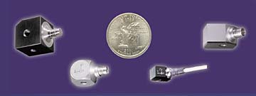 Most piezoelectric accelerometers are made of quartz crystal, piezoelectric ceramics, or, for high-temperature operation, tourmaline or lithium niobate. They obey Newton's second law, F = ma, in that the force acting on the measuring element is directly proportional to the acceleration produced. Available in a wide range of configurations and operating specifications, these devices are used wherever shock or vibration is of interest. |
The charge amplifier principle was patented by W.P. Kistler in 1950 and gained practical significance in the 1960s. The introduction of MOSFET solid-state circuitry and the development of highly insulating materials such as Teflon and Kapton greatly improved performance and propelled the use of piezoelectric sensors into virtually all areas of modern technology and industry.
Piezoelectric measuring systems are active electrical systems. That is, the crystals produce an electrical output only when they experience a change in load?they cannot perform true static measurements. However, it is a misconception that piezoelectric iýstruments are suitable for only dynamic measurements. Quartz transducers, when paired with adequate signal conditioners, offer excellent quasistatic measuring capability. There are countless examples of applications where quartz-based sensors accurately and reliably measure quasistatic phenomena for minutes and even hours.
There are two types of piezoelectric sensor: high and low impedance. High-impedance units have a charge output that requires a charge amplifier or external impedance converter for charge-to-voltage conversion. Low-impedance types use the same piezoelectric sensing element as high-impedance units and also incorporate a miniaturized built-in charge-to-voltage converter. They also require an external power supply coupler to energize the electronics and decouple the subsequent DC bias voltage from the output signal.
Quartz-Based Piezoelectric Sensors
Although this article focuses on accelerometers, the response function for force and pressure sensors is nearly identical. In fact,
|
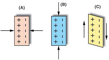
Quartz piezoelectric sensors consist essentially of thin slabs or plates cut in a precise orientation to the crystal axes depending on the application (see Figure 1, and "The Piezoelectric Effect in Crystals"). Most Kistler sensors incorporate a quartz element that is sensitive to either compressive or shear loads. The shear cut is used for multicomponent force and acceleration measuring sensors. Other specialized cuts include the transverse cut for some pressure sensors and the polystable cut for high-temperature pressure sensors.
The finely lapped quartz elements are assembled either singly or in stacks and preloaded in some manner. The quartz package generates a charge signal, measured in picoCoulombs, that is directly proportional to the sustained force. Each sensor type uses a quartz configuration optimized and ultimately calibrated for its particular application (e.g., force, pressure, acceleration, or strain).
Of the large number of piezoelectric materials available today, quartz is preferred in sensor designs because of the following properties:
- Material stress limit of ~20,000 psi
- Temperature resistance up to 930°F
- Very high rigidity, high linearity, and negligible hysteresis
- Almost constant sensitivity over a wide temperature range
- Ultra-high insulation resistance (1014
 ), allowing low-frequency measurements (<1 Hz)
Dynamic Behavior
 |
(1) |
where:
| fn | = | undamped natural (resonant) frequency (Hz) |
| f | = | frequency at any given point of the curve (Hz) |
| ao | = | output acceleration |
| ab | = | mounting base or reference acceleration (f/fn = 1) |
| Q | = | factor of amplitude increase at resonance |
Quartz sensors have a Q of ~10?40; the phase angle can therefore be written as:
 |
(2) |
As can be seen in a typical frequency response curve (see Figure 2), an amplitude rise of ~5% can be expected at ~1/5 of fn.
 Figure 2. In this typical response curve, 1 = low-frequency limit determined by RC rolloff characteristics; 2 = usable range; 3 = high-pass filter; and 4 = with low-pass filter, which can be used to attenuate the effects of the amplitude rise at ~1/5 the resonance frequency. |
Low-pass filtering can be used to attenuate the effects of this. Many Kistler signal conditioners (charge amplifiers and couplers) have plug-in filters for this purpose.
Charge Amplifiers
Basically the charge amplifier consists of a high-gain inverting voltage amplifier with a MOSFET or JFET at its input to achieve high insulation resistance (see Figure 3).
 Figure 3. The charge amplifier consists of a high-gain inverting voltage amplifier with a FET at its input for high insulation resistance. In this simplified schematic, 1 = accelerometer; 2 = charge amplifier; Vo = output voltage; A = open-loop gain; Ct = sensor capacitance; Cc = cable capacitance; Cr = range (or feedback) capacitor; Rt = time constant resistor (or insulation resistance of range capacitor); Ri = insulation resistance of input circuit (cable and sensor); and q = charge generated by sensor. |
 |
(3) |
where:
| q | = | charge generated by the sensor |
| Cr | = | range capacitor |
| Ct | = | sensor capacitance |
| Cc | = | cable capacitance |
| A | = | open-loop gain |
For sufficiently high open-loop gain, the cable and sensor capacitance can be neglected, leaving the output voltage dependent only on the input charge and the range capacitance:
| (4) |
In short, the amplifier acts as a charge integrator that compensates the sensor's electrical charge with a charge of equal magnitude and opposite polarity, and ultimately produces a voltage across the range capacitor. In effect, the purpose of the charge amplifier is to convert the high impedance charge input, q, into a usable output voltage, Vo.
Time Constant and Drift. Two of the more important considerations in the practical use of charge amplifiers are time constant and drift. The time constant (TC) is defined as the discharge time of an AC-coupled circuit. In a period of time equivalent to one time constant, a step input will decay to 37% of its original value. The TC of a charge amplifier is determined by the product of the range capacitor, Cr, and the time constant resistor, Rt:
| (5) |
Drift is defined as an undesirable change in output signal over time that is not a function of the measured variable. Drift in a charge amplifier can be caused by low insulation resistance at the input, Ri, or by leakage current of the input MOSFET or JFET. Drift and time constant simultaneously affect a charge amplifier's output. One or the other will be dominant. Either the charge amplifier output will drift toward saturation (power supply) at the drift rate, or it will decay toward zero at the time constant rate.
Many Kistler charge amplifiers have selectable time constants that are altered by changing the time constant resistor Rt. Several of these charge amplifiers have a short, medium, or long time constant selection switch. In the long position, drift dominates any time constant effect. As long as the input insulation resistance Ri is maintained at >1013![]() , the charge amplifier (with MOSFET input) will drift at an approximate rate of 0.03 pC/s. Charge amplifiers with JFET inputs are available for industrial applications but have an increased drift rate of ~0.3 pC/s. In the short and medium positions, t°e time constant effect dominates normal leakage drift. The actual value can be determined by referring to the appropriate operation/instruction manual supplied with the unit.
, the charge amplifier (with MOSFET input) will drift at an approximate rate of 0.03 pC/s. Charge amplifiers with JFET inputs are available for industrial applications but have an increased drift rate of ~0.3 pC/s. In the short and medium positions, t°e time constant effect dominates normal leakage drift. The actual value can be determined by referring to the appropriate operation/instruction manual supplied with the unit.
Frequency and Time Domain Considerations. When considering the effects of time constant, the user must think in terms of either frequency or time domain. The longer the time constant, the better the low-end frequency response and the longer the usable measuring time. When measuring vibration, time constant has the same effect as a single-pole, high-pass filter whose amplitude and phase are:
 |
(6) |
 |
(7) |
For example, the output voltage has declined ~5% when f × (TC) = 0.5 and the phase lead = 18°. When measuring events with wide (or multiple) pulse widths, the time constant should be at least 100 × longer than the total event duration. Otherwise, the DC component of the output signal will decay toward zero before the event is completed.
Other design features incorporated into Kistler charge amplifiers include range normalization for whole number output, low-pass filters for attenuating sensor resonant effects, electrical isolation for minimizing ground loops, and digital/computer control of setup parameters.
Low-Impedance Piezoelectric Sensors
Piezoelectric sensors with miniature, built-in charge-to-voltage converters are identified as low-impedance units for our purposes here. These units incorporate the same types of piezoelectric sensing element(s) as their high-impedance counterparts.
In 1966, Kistler developed the first commercially available piezoelectric sensor with internal circuitry. This circuit, of a patented design called the Piezotron, incorporates a miniature MOSFET input stage followed by a bipolar transistor stage and operates as a source follower (unity gain). These elements are incorporated in a monolithic IC. The circuit has an input impedance of
1014![]() and output impedance of 100
and output impedance of 100 ![]() , which allows the charge generated by the quartz element to be converted into a usable voltage. The Piezotron design requires only a single coax for power-in and signal-out. Power to the circuit is provided by a coupler that supplies a 2?18 mA source current and a 20?30 VDC energizing voltage (see Figure 4).
, which allows the charge generated by the quartz element to be converted into a usable voltage. The Piezotron design requires only a single coax for power-in and signal-out. Power to the circuit is provided by a coupler that supplies a 2?18 mA source current and a 20?30 VDC energizing voltage (see Figure 4).
 Figure 4. All that is needed to operate a Kistler low-impedance accelerometer are a coupler and coax cable. Here, 1 = accelerometer; 2 = coupler, 3 = decoupling capacitor; 4 = constant-current diode; 5 = reverse polarity protection diode; q = charge generated by piezoelectric element; Vi = input signal at gate; Vo = output voltage (usually bias decoupled); Cq = sensor capacitance; Cr = range capacitance; CG = MOSFET gate capacitance; and Rt = time constant resistor. |
The steady-state output voltage is essentially the input voltage at the MOSFET gate plus any offset bias adjustment. The Piezotron's voltage sensitivity can be approximated by:
| (8) |
The range capacitance, Cr, and time constant resistor, Rt, are designed to provide a predetermined sensitivity (mV/g) and upper and lower usable frequencies. The exact sensitivity is measured during calibration and its value is recorded on each unit's calibration certificate.
Time Constant. The time constant of a Piezotron or similar quartz accelerometer is:
| (9) |
Time constant effects are the same in low-impedance sensors and charge amplifiers. That is, both act as a single-pole, high-pass filter as discussed previously.
Low-Impedance Power Supply
For excitation of their integral electronics, low-impedance accelerometers require only a single coaxial cable and a power supply coupler. Both the power into and the signal out of the sensor are transmitted over this cable. The coupler provides the constant current excitation required for linear operation over a wide voltage range and also decouples the bias voltage from the output.
Time Constant. Bias decoupling methods can be categorized as AC or DC. DC decoupling will not affect a low-impedance sensor's time constant and therefore permit optimum low-frequency response. An offset voltage adjust is used to "zero" the bias. AC decoupling methods, however, can shorten the low-impedance sensor's time constant and degrade low-frequency response. In low-impedance systems with AC bias decoupling, the system time constant can be approximated by taking the product of the sensor and coupler time constants and dividing by their sum. The resulting frequency response can be computed as before.
Comparing High- and Low-Impedance Systems
Similarities.ðBoth use the same type of piezoelectric sensing element(s) and are therefore AC-coupled systems with limited low-frequency response or quasistatic measuring capability. Their respective time constants determine the usable frequency range.
High Impedance. These are typically more versatile than low-impedance systems. Time constant, gain, normalization, and reset are all controlled by means of an external charge amplifier. In addition, high-impedance systems usually have longer time constants that allow easy short-term static calibration. With no built-in electronics, they have a wider operating temperature range.
Low Impedance. In general, low-impedance systems are tailored to a particular application. Since these sensors have an internally fixed range and time constant, their use might be limited to a particular application. There is no such restriction on high-impedance systems, where range and time constant are controlled with an external charge amplifier. For applications with well-defined measuring frequency and temperature ranges, however, low-impedance systems can cost less and furthermore can be used with general-purpose cables in environments where high humidity and/or contamination could be detrimental to the high insulation resistance required for high-impedance sensors. Also, longer cable lengths between sensor and signal conditioner and compatibility with a wide range of signal display devices are further advantages of low-impedance sensors.
An alternative method for processing charge from high-impedance sensors is to use an external impedance converter, which exploits the high temperature range of the sensor while offering the convenience and cost-effectiveness of a coupler, as compared to a charge amp.
Applications of Piezoelectric Accelerometers
Piezoelectric measuring devices are widely used today in the laboratory, on the production floor, and as original equipment for measuring and recording dynamic changes in mechanical variables including shock and vibration. The following is only a partial list:
- Aerospace. Modal testing, wind tunnel, and shock tube instrumentation; landing gear hydraulics; rocketry; structures; ejection systems
- Ballistics. Combustion, explosion, and detonation
- Engine Testing. Combustion and dynamic stressing
- Engineering. Materials evaluation, control systems, reactors, structural analysis, auto chassis structural testing, shock and vibration isolation, and dynamic response testing
- Industrial/Factory. Machining systems, metal cutting, and machine health monitoring
- OEMs. Transportation systems, rockets, machine tools, engines, flexible structures, and shock/vibration testers
|