
You're in a dark corner of your basement holding a bucket of water. Water is streaming from a hole in the side of the bucket. Trying to find the hole, you grab a flashlight and shine it into the bucket. What do you see? A glowing stream of water coming from the hole. What's going on here? How does the light stay within that stream of water?
This situation demonstrates the basis of fiber-optic sensing and fiber-optic communications: Photons tend to stay within a conduit when its index of refraction (or dielectric constant) is higher than that of the surrounding materal. When considering concentric regions of dielectric media with slightly differing indices of refraction, total internal refection of an electromagnetic wave causes the wave to behave as if it were bouncing down a light pipe.
Measuring with Light | |
| Part 1 | |
| Part 2 | |
| Part 3 | |
| Part 4 | |
• More light can be coupled into a multimode fiber (because of its larger core).
• Multimode fibers typically experience more signal loss due to more scattering centers in the larger core.
• Multimode fibers exhibit more signal distortion because of the multiple paths that the light signal can take as it proceeds along the larger fiber.
• Single-mode fibers provide more spatial control of the optical field, resulting in significantly less distortion and less signal loss.
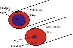 |
| Figure 1. These drawings show the two general categories into which optical fibers fall. The core of a multimode fiber is considerably larger than that of a single-mode fiber. The diameter of a typical single-mode core is in the 4–9 micron range; the multimode core measures from 50 microns to the millimeter range. |
• When coherent (i.e., laser) light is coupled into the fibers, the output of a multimode fiber will exhibit a spatial graininess, but a single-mode fiber's output will look like a single dot.
While there are variations, the outside diameters of single-mode and multimode fibers tend to be ~125 microns (or about the size of a strand of hair). To the touch, it's impossible to distinguish between the two modes. When the size exceeds 125 microns (fibers can be up to a millimeter in diameter), the fibers are strictly multimode.
A buffer jacket protects the fiber from harmful chemicals. When many fibers are used to form a cable, each buffer can be a different color, allowing you to distinguish one from another at each end of the cable. If you suspect that the fiber is going to be placed in a hazardous environment, you can wrap the core/cladding/buffer fiber sandwich with a Kevlar braid and then encase everything in a plastic housing.
How and Why Optical Fibers Guide Light
But why does the light stay in the fiber? This isn't just an academic question. By understanding some of these details, you can understand how fiber-optic sensors and communications systems work. The propagation phenomenon lies in the realm of electromagnetic (EM) field theory and the interaction of an EM field at an interface between two dielectric media.
Consider an EM wave that is incident on the interface of two dielectric media. The two components of the field are the electric and magnetic intensity vectors:
![]()
![]()
E0 is a vector whose amplitude is time independent and whose direction is tangential to the direction of propagation. The direction that the incoming field is traveling in is mathematically given as k0, which is the wave vector (or propagation vector) whose direction is normal to the propagating wavefront. In other words, the electric and magnetic fields lie in a flat sheet perpendicular to the direction that the wavefront is propagating. If a rectangular coordinate system is oriented along the interface (see Figure 2), the traditional angles of incidence (i.e., reflection and refraction) can also be defined with respect to a line that is perpendicular to the interface. Other important terms from Equations 1 and 2 include the amplitude of the wave vector:
![]()
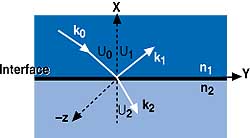 |
| Figure 2. The interface geometries between two dielectric media set the stage for how the electromagnetic wave will behave. In this diagram, the X axis points straight up, the +Y axis runs to the right, and the –Z direction points straight out of the page right at you. |
where:
r = the position vector for an arbitrary
point in space
ω = the radian frequency of the EM wave
The reflected and transmitted waves are expressed in a manner similar to Equations 1 and 2:
kkk
kkkk
kkkk
Reflected,
![]()
![]()
Transmitted,
![]()
![]()
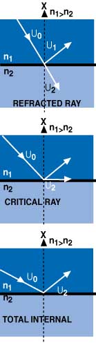 |
| Figure 3. This diagram shows the geometry used to mathematically describe and predict how an electromagnetic wave will behave at an dielectric interface. Total internal reflection of a wave happens when the angle becomes so steep that Snell's Law breaks down (it predicts a sine value >1—nope!), with the only acceptable solution requiring that a total phase change occur. In other words, total internal reflection must happen. |
Empirical and mathematical investigations by Faraday, Gauss, and Ampere led to a suite of laws, summarized by James Clerk Maxwell, that guide us in understanding what happens at the boundary of the two dielectric media. The application of Gauss's law at a dielectric boundary tells us that the normal (i.e., perpendicular) component of the electric field is continuous across the boundary. In mathematical terms, this normal field component boundary condition is:
![]()
And what about the tangential electric field component, the part of the field that lies along the interface boundary? In a source-free region (e.g., the dielectric interface), but not for metallic interfaces, Maxwell's equations are expressed as:
![]()
![]()
Applying mathematical trickery using Stokes' theorem and then doing the integral over the perimeter of a bounding area leads to the boundary condition for the electric field tangential components: they must be continuous across the boundary between the two media. Similarly, noting that there is no divergence to a magnetic field,
![]()
you get
![]()
A realistic interpretation of Equation 12 shows that the tangential components of the magnetic induction vector, B, are also continuous across this dielectric boundary. Returning to the geometry shown in Figure 3, all wave vectors are in the plane of incidence, or coplanar, which gives us the following equalities:
![]()
Total internal reflection means that the reflected wave and the incident wave are in the same medium:
![]()
Apply this to Equation 3,
![]()
and voila, a 17th century optics equation is found:
![]()
From Equation 13, you gain an insight into the properties of optical fibers. Once again, consider Figure 3, and in particular, examine the input and output angles from this interface, θ0 and θ2. What happens when θ2=π/2 (the reflected angle equals 90°)? In this case, sin θ2 = 1, and Snell's law can be rewritten as:
![]()
Because the sine of a nonimaginary angle can never be >1, this forces n1 >n2, and
![]()
It would seem from Figure 3 that when
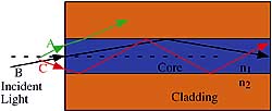 |
| Figure 4. If light enters the core at too steep of an angle, it is not totally internally reflected from the core-cladding interface. Light that enters the core within the acceptance angle can take different paths as it bounces down the multimode light pipe. |
θ2 > π/2 there is no longer any transmitted light through the interface, as k2 points along the boundary itself. In other words, the light is totally reflected. This provides some guidance for the situation: if n2 > n1, you get external reflection, but total internal reflection demands that n1 > n2.
The index of refraction of the core material must be larger than the index of refraction of the cladding material. The angle q0 in Equation 18 is called the interface's critical angle. Transferring the critical angle at the core-cladding interface to the front surface of the fiber results in the acceptance angle of the fiber. If the angle of the input EM wave is larger than the accceptance angle (see Figure 4), the incident light will not be totally internally reflected and will enter the cladding, causing it to glow. If the angle of the incident light is less than the acceptance angle, the light is guided in this dielectric sandwich. Once light is inside the optical fiber, it will propagate along the fiber and around bends for kilometers with minimal loss.
Characteristics of Optical Fibers
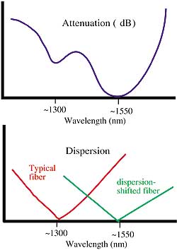 |
| Figure 5. (A) shows the attenuation versus wavelength of light propagating in a single-mode optical fiber. (B) shows the amount of pulse spreading (or dispersion) for typical and dispersion-shifted single-mode fiber, with respect to the wavelength of the light propagating down the fiber. |
While you can model the attenuation of light in an optical fiber as a damped exponential, the actual process in terms of the overall attenuation of the signal is quite complex, involving scattering, absorption, and imperfect reflections. Transmission characteristics depend on the wavelength of the light propagating in the fiber. For a standard telecommunications grade fiber, the minima in attenuation occur in the 1300 nm and 1550 nm windows (see Figure 5a).
Attenuation is important for the light guide. If the signal level drops too low, well, you get the picture. Therefore, if the light source operates in the fiber's attenuation window, then other fiber-induced effects can become dominant—most notably, dispersion. Dispersion in the fiber (resulting in pulse spreading) arises from a variety of effects:
• Chromatic dispersion is caused by the use of a relatively wide spectral source (e.g., an LED). You can compensate for this by using a single longitudinal mode laser (fewer colors—less chromatic dispersion).
• Modal dispersion is caused by the optical field taking different length paths through the fiber. You can eliminate this form of dispersion by using single-mode fiber (only one path through the fiber—no modal dispersion).
• Finally, consider the case in which a square pulsed data signal propagates down a fiber. The laser source—even if it is deemed to be in the single longitudinal mode—has spectral width. Each color found in the signal sees slightly different values of material dispersion and propagates at different speeds. This results in pulse spreading. A Fourier decomposition of the pulsed data sequence reveals that the optical carrier is itself being slightly frequency modulated because of the spectral components of the data pulse. Even this seemingly small effect leads to dispersion because the optical fiber manifests different indices of refraction values for these frequencies. This form of dispersion limits the overall performance of the communications system, because you can minimize it (e.g., don't transmit square pulses), but you can't easily eliminate it.
An expression for the material dispersion coefficient is determined considering unit distance and substituting w = 2πc/λ:
![]()
c dl2
For silica-based optical fiber, the dispersion coefficient, Dmλ, is equal to zero at a wavelength of about 1300nm. Below the wavelength, the coefficient assumes values lower than zero, whereas above 1300 nm, the sign is reversed.
In standard optical fibers, the waveguide dispersion component is relatively important when it is near 1300nm, when the material dispersion is negligible. The field amplitude distribution depends on the refractive index profile, which can be tailored in the fiber design to shift the zero in the total dispersion toward longer wavelengths (e.g., 1.55 µm). The waveguide dispersion coefficient, Dwλ, can be given by:
![]()
Because b depends on both V and l, the same dependence is for Dwλ. This confirms that it is possible to control the waveguide dispersion by acting on the refractive index profile.
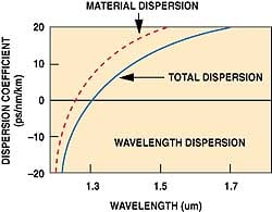 |
| Figure 6. This graph shows the total chromatic dispersion for a standard, single-mode, telecommunications-grade optical fiber. In certain instances, it's possible to balance the positive material and the negative waveguide dispersion characteristics to yield a total signal dispersion that approaches 0, resulting in no pulse spreading. |
Review of Figure 5 indicates that for typcal fiber the attenuation minimum occurs at 1550 nm, and the minimum in dispersion occurs near 1300 nm. It's too bad that those two minima don't overlap in the same wavelength band.
But wait. As shown in Figure 6 , Dmλ and Dwλ have opposite signs—one is negative, and the other is positive. Therefore, the core index profile can be tailored to obtain a shift of the zero dispersion wavelength l0. Furthermore, the index profile of the optical fiber can be shaped to obtain a dispersion-flattened fiber in which the total chromatic dispersion coefficient is small over a broad wavelength range covering the low attenuation windows.
Conclusion
In terms of attenuation and dispersion, what guidance does this analysis provide? For lowest loss, the light source should emit in the 1550 nm range; for minimal dispersion, use a laser operating at 1300 nm. But if you've obtained dispersion-shifted fiber, then use a laser operating at 1550 nm, and by all means don't send square pulses down the fiber. Round those edges (use a raised cosine filter) to reduce the dispersion effects. To really reduce the dispersion, use single-mode fiber. The entrance pupil is small, so you'll have a tougher time coupling light into the fiber, but once it's in there, it'll go seemingly forever.
Editor's Note
The information in this series of articles will be included in Dr. Fuhr's tutorial “Fundamentals of Fiber-Optic Sensing: Techniques, Applications, and More Applications," which will be presented in the Sensors Expo Conference Program in Anaheim, CA, on May 9, 2000.