
The linear variable differential transformer (LVDT) has been around for many years, and remains a popular sensing technology for absolute position measurement. It is relatively simple, operates over a wide temperature range, has extremely fine resolution, never wears out, and has high reliability. It is well suited for linear measurements over ranges from microns to several inches, but becomes less cost-effective at stroke lengths greater than ±3 in.
Differential transformers have been used in various forms since the 1930s, and the LVDT became widely known in the 1940s when Herman Schaevitz published his paper, "The Linear Variable Differential Transformer," [1]. The LVDT became more prevalent as an industrial sensor in the 1960s with the advent of solid-state electronics. It is still popular today, having undergone many improvements in performance and having been adapted for the miniaturization of the associated electronics.
Basic Configuration
The basic LVDT (see Figure 1) comprises three axially aligned stationary coils having a central bore, and a core that is movable within the bore. There is enough clearance between the core and the bore to prevent them from contacting each other. The center coil is the primary of the transformer, and is driven by an AC waveform at a constant frequency of 50 Hz to >10 kHz. The most popular operating frequency is 2.5 kHz. The two secondary coils are wired in series-bucking, so that their voltages subtract.
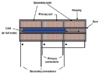 Figure 1. The basic configuration of an LVDT comprises three coils and a movable core. |
Operation
When the core is centered, an equal voltage amplitude is induced across each secondary by transformer action. But since the secondaries are wired in series-bucking, the phases of the two voltages are opposite, thus producing a theoretical output of zero V. When the core is centered, it is called the null position (see Figure 2).
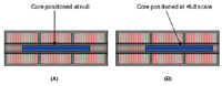 Figure 2. An LVDT is shown with the core positioned at null (A) and at full scale (B). |
Although the output voltage at null is theoretically zero, there remains a small AC null voltage. The exact position of the null is where the sum of the outputs of the two secondaries is at its lowest value [2]. The null voltage, however, is insignificant after demodulation. When the core moves to one side of null, the voltage across that coil increases as the other decreases. This results in a steadily increasing voltage across the output leads. This AC voltage is usually rectified or demodulated to produce a DC output voltage that increases with the distance of the core from null, and with a polarity (positive or negative) that indicates the direction of travel from null. So, for example, an LVDT with a range of ±1.000 in. could be demodulated to provide a DC output signal of ±1.000 V. Then the output would linearly change from +1 V at +full scale of +1.000 in., down to zero V at null, and then continue to –1.000 V when it reaches negative full scale.
Since the core is coupled to the coils inductively, there is no need for any mechanical contact between the moving core and the stationary parts (e.g., coils, housing). The LVDT is therefore a noncontact position sensor, which means it can be used in applications that have continuous motion and there will be no worry of its ever wearing out. If a mechanical assembly is used for alignment of the core assembly, however, then the assembly should be evaluated for any lifetime limitations due to wear (see Figure 3).
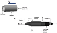 Figure 3. A typical LVDT has a cylindrical housing and separate core (A). An LVDT of the gauge head configuration has a built-in core assembly (B). |
The LVDT is an absolute position sensor, providing a reading of distance from a fixed datum, rather than from a previous position. This is important in high-noise industrial environments, and ensures that the correct signal will be present after externally induced corruption of the measurement data.
The LVDT in Figure 3(B) is called a gauge head configuration. It includes a mounting thread, a core holder that may include a spring or air pressure return, and linear bearings that provide for core alignment. The gauge head configuration has the advantages of easy mounting and alignment. Even though there may eventually be some wear of the mechanical elements, this does not affect the accuracy of the sensor.
The LVDT core is fabricated from a nickel-iron alloy, formulated to provide relatively high permeability for induction and heat treated to ensure uniform permeability along its length. The core usually has an internal thread for mounting. For uniform permeability, the heat-treating must take place after the core is cut to length and threaded. A core extension rod is normally connected between the core and the member to be measured. The core extension rod must be fabricated from material with low magnetic permeability, such as plastic, aluminum, brass, or some stainless steels.
Circuitry
The circuitry used to operate an LVDT is often called the conditioning circuit, or the signal conditioner. A typical conditioning circuit would include a voltage regulator, sine wave generator, demodulator, and an amplifier (see Figure 4).
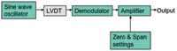 Figure 4. The elements of an LVDT signal conditioner are shown in this block diagram. |
It is important that the sine wave generator have a constant amplitude and frequency, unaffected by time or temperature. A sine wave can be produced by a Wien bridge circuit, by filtering a square wave or staircase wave, or by other suitable methods. Some representative circuits are shown in Figure 5.
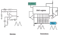 Figure 5. A suitable sine wave to drive the LVDT primary can be produced by using a Wien bridge circuit or by filtering a staircase waveform. |
The demodulator may be a simple diode configuration or a synchronous demodulator (see Figure 6). The simple diode demodulator in Figure 6(A) may be used when the AC output voltage from the LVDT secondaries is >1 V F.S. If the signal voltage is lower than that, there may be a temperature sensitivity problem due to differences in the forward voltages between the two diodes. With a higher signal voltage, the diode error is less noticeable.
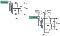 Figure 6. A simple diode demodulator can be used (A), or one with synchronous demodulation (B). |
In the synchronous demodulator of Figure 6(B), the two field effect transistor switches alternately turn on and off with timing that is synchronous with the sine wave that powers the primary. The amount of phase shift required between the primary and the demodulator switches depends on the LVDT specification and on the length of the leads between the LVDT and the signal conditioner.
Sine wave generator, demodulator, and amplifier circuits have been combined into commercially available ICs for more than 20 years. Using one of these components will substantially simplify the design of an LVDT signal conditioner. The most popular are the NE5521 from Philips (www.philipsusa.com), and the AD 598/698 series from Analog Devices Inc. (www.analog.com). The Philips NE5521 has been recently discontinued, however, reportedly due to the loss of the mask in a fire. The Analog Devices parts are well proven, but somewhat expensive. Alternatively, with the advent of standard analog and digital device availability in fine-pitch packages, the circuitry can be designed from scratch and still fit inside an LVDT housing.
Technology Comparison
As previously noted, the LVDT has many excellent qualities. Its principal limitations are the need for the sensor housing to be longer than the stroke length for linear performance, and the nonlinearity of the output signal vs. input measurand. Some of the typical performance parameters of an LVDT and the way they compare to other technologies are shown in Figure 7.
 Figure 7: Comparison of Technologies. |
Both the ratio of stroke length to housing length and the nonlinearity problem can be ameliorated with special conditioning techniques, one of which is to add a microcontroller to make corrections. This is possible because the LVDT has very good repeatability.
LVDTs are also available as rotary devices. They operate in a fashion similar to that of the linear models, but have shaped cores that move over a curved path. They are typically available for full-scale travel of up to 120° of rotation. Figure 8 lists some LVDT and/or signal conditioner suppliers and their URLs.
 Figure 8: LVDT and Signal Conditioner Suppliers. |
Summary
Although LVDTs have been around for a long time, they are still a demonstrated solution to many position sensing problems. Their robust construction provides high reliability, while their performance is well-suited to most applications with less than ±3 in. of travel. Keep them in mind for your next position sensing application.
References
1. Herceg, Edward E., Handbook of Meas-urement and Control, 1976, Schaevitz Engineering, Pennsauken, NJ, pp. 3–4.
2. Nyce, David S., Linear Position Sensors,
Theory and Application, 2004, John Wiley and Sons, Hoboken, NJ, p. 96.
David S. Nyce, B.S.,E.E., can be reached at Revolution Sensor Company, Apex, NC; 919-362-6923, [email protected], www.rev.bz.