
Part 1 of this article discussed the importance of sensing small magnetic fields in industrial and medical applications. It explained the physical concepts behind giant magnetoresistance (GMR) and compared the properties of several types of GMR materials. This part shows how these materials function in low magnetic field sensing and discusses things you should consider when using GMR sensors, including noise, amplification, magnetic biasing, and sensor arrays. To illustrate these points, several low-field applications of present and future GMR sensors are discussed. The figures and references in Part 2 are numbered consecutively from those in Part 1.
GMR Sensors
Thin-film GMR materials deposited on silicon substrates can be configured as resistors, resistor pairs or half bridges, and Wheatstone bridges. A sensitive bridge can be fabricated from four photolithographically patterned GMR resistors, two of which are active elements. The sheet resistance of the thin films is between 10 (omega) and 15 (omega) per square. Resistors of 10 k(omega) can be formed as 2 µm serpentine traces covering less than a 100 µm square. Small magnetic shields of permalloy plated over two of the four equal resistors in a Wheatstone bridge--the resistor connected to power on one side and the resistor connected to ground on the other side--protect the resistors from the applied field and let them act as reference resistors.
Because they are made of the same material, the reference resistors have the same temperature coefficient as the active resistors. The two remaining GMR resistors are exposed to the external field. The bridge output is therefore twice the output you would expect of a bridge with only one active resistor. The bridge output for a 10% change in these resistors is ~5% of the voltage applied to the bridge.
Additional permalloy structures plated onto the substrate can act as flux concentrators to increase sensitivity. The active resistors are placed in the gap between two flux concentrators. These resistors experience a field larger than the applied field by approximately the ratio of the gap between the flux concentrators to the length of one of the flux concentrators. In some sensors, the flux concentrators are also used as shields by placing two resistors beneath them.
The sensitivity of a GMR bridge sensor can be adjusted in design by changing the lengths of the flux concentrators and the gap between them. In this way, a GMR material, which saturates at ~300 Oe, can be used to build different sensors, which saturate at 15 Oe, 50 Oe, and 100 Oe. To produce sensors with more sensitivity, external coils and feedback can be used to produce sensors with resolution in the 100 mA/m or millioerstead range.
An example of the output from a low-field GMR bridge sensor is shown in Figure 6 (page 85). The curve traces out a full bipolar excitation of the sensor. The bipolar hysteresis shown is only observed when the sensor crosses from a large negative excursion to a positive excursion or vice-versa. The unipolar hysteresis is shown by the two lines on each side, which almost coincide. This sensor has a bridge resistance of 5 k(omega) and a slope sensitivity of 3.7 mV/V/Oe. The flux concentrators on this sensor provide a gain of ~16. The size of the sensor die is 0.44 mm by 3.37 mm, and it is packaged in an 8-pin SIOC package, with a footprint of 6 mm by 4.9 mm.
Wheatstone bridge sensors can also be made from spin-dependent tunneling (SDT) material, which was described in Part 1 of this article. Because of the insulating layer, high resistances can be obtained in small areas. SDT sensors operate in a hysteretic or linear mode, depending on the sensing application. With no current passed through the integrated biasing straps, the output has an open shape with considerable hysteresis. This mode is useful for on/off types of applications in which you want a large signal change to occur at fields above a certain level, say ±1 Oe. This type of output is shown as the dotted line in Figure 7 (page 86). The switching threshold for this curve can be adjusted by changing the length of the flux concentrators. With ~40 mA of current through the integrated biasing coil, the output becomes linear, with a lower slope and much less hysteresis. This mode is ideal for sensing small changes in the magnetic field. Sensor output using this mode of operation is shown as the solid line in Figure 7.
 |
| Figure 6. The output from a low magnetic field GMR Wheatstone bridge sensor under bipolar excitation shows its omni-polar, or pole-indifferent, response. The hysteresis near the origin is greatest if the sensor is traversed from large positive magnetic fields to large negative fields and back to large positive fields. |
These sensors are still under development. Table 1 shows the preliminary operating parameters of Wheatstone bridge STD sensors.
When working with SDT material, manufacturers can make sensors with a wide range of resistance values using the same footprint. The 5–50 k(omega) specifications shown in Table 1 are in the lower end of the resistance range. If an application requires a higher resistance, sensors with resistances as high as 10 M(omega) are easy and economical to make.
Circuit Considerations
The ultimate limitation on low magnetic field sensing is noise. If the SNR is <1, you'll have a hard time getting a meaningful measurement. Fortunately, there are several methods of improving the SNR if you understand the sources of the noise [10].
You can divide noise into two categories: inherent and transmitted. The sensor and the sensing system produce inherent noise. Transmitted noise is introduced into the sensing system from the outside world. Inherent noise can include such things as sensor and amplifier offset, thermal noise, and 1/f noise. Transmitted noise includes magnetic fields from unwanted sources and electrical noise from external sources picked up by the sensing system.
| TABLE 1 | |
| Sensor type: | Wheatstone bridge |
| Linear field range: | ±0.5 Oe |
| Output vs. field polarity: | Bipolar |
| Voltage sensitivity: | ~10–100 mV/V/Oe |
| High-frequency noise floor: | ~10–100 nOe/(check)Hz |
| Noise at 1 Hz: | ~1–10 mOe/(check)Hz |
| Saturation field: | ±1.0 Oe |
| Bridge resistance: | 5–50 k |
| Max. bridge power: | 2–20 mW |
| Flux concentration: | 10 x |
| Die size: | 1.65 mm by 2.14 mm |
| Operating temperature range: | –40°C to 185°C |
| Max. operating voltage: | 15 V |
Thermal noise is associated with random thermal motions at the atomic level. Because the noise is uniform with frequency, the noise voltage in a given bandwidth is proportional to the square roots of the resistance, temperature, and bandwidth. At room temperature, the noise voltage divided by the square root of the bandwidth is 0.13 (check)R (nV/(check)Hz) or 9 nV/(check)Hz for a 5 k(omega) sensor. To minimize thermal noise, limit the bandwidth to the frequencies of the magnetic signal of interest and use small resistors. The resistance of the sensing resistor itself may, however, be constrained by power and amplification considerations.
 |
| Figure 7. The output from a spin-dependent tunneling bridge sensor under bipolar excitation shows hysteresis and high slope gain near the origin in the dashed curve with no bias applied. Applying a bias field via coils reduces both the hysteresis and slope gain. |
A second source of inherent noise in all conductors is 1/f noise. This noise is caused by point-to-point fluctuations of the current in the conductor [11], is proportional to the inverse of the frequency, and often dominates below 100 Hz. Our best estimates for the 1/f noise in a 5 k(omega) multilayer GMR sensor is 300 nV/(check)Hz at 1 Hz and 1 mA.
At the lowest frequencies, it's difficult to distinguish 1/f noise from drift. Although thermal noise is independent of current and exists even without it, the 1/f noise is proportional to the current and increases as the current grows. Bandwidth limitation, especially on the low-frequency end, will reduce 1/f noise. As with any random noise source, averaging a repetitive signal will increase the SNR by the square root of the number of singles averaged.
Transmitted noise sources include voltages picked up by the circuit and magnetic readings acquired by the sensor that are not part of the desired magnetic signal. A time-varying magnetic field will not only produce a signal in a magnetic sensor, it will also induce a voltage in a circuit loop proportional to the circuit loop area and the time rate of change of the magnetic field. To minimize the inductive pick up, you must follow good circuit practices, including minimizing circuit loops and placing amplification as close to the sensor as possible.
Electrical currents generate magnetic fields, and you can usually find stray 60 Hz magnetic fields in any industrial location. The growing use of computers and other equipment with rectifier-fed, capacitor-input power supplies produces an increasing number of nonsinusoidal currents that generate 60 Hz harmonics. Any moving or rotating magnetic material in equipment will produce a time varying magnetic field at frequencies characteristic of their period.
The Earth's magnetic field and its slow random variation produce noise that can interfere with the monitoring of low-frequency magnetic fields. You can best minimize transmitted magnetic noise by filtering and, if practical, by using magnetic shielding. When measuring fields from a dipole source close to a sensor, you can locate a second sensor at least twice as far from the dipole. The difference between the two signals, when adjusted for differences in sensitivity, will be at least 7/8 the signal while canceling out the signals from remote sources.
 |
| Figure 8. On the left, a sensor is back biased by a permanent magnet attached to its top side. Due to the positioning of the magnet, there is little or no magnetic field in the horizontal direction, the sensor's sensitive axis. On the right, the influence of a ferromagnetic object is shown. By attracting the magnetic field lines from the permanent magnet, the object produces a horizontal component of field, which is sensed by the sensor. |
Instrumentation amplifiers work well with low-field Wheatstone bridge GMR sensors. When combined with an operational amplifier, the sensor/amplifier easily achieves gains of several thousand. You can also incorporate high-pass and low-pass filters formed from passive components in the circuit to limit noise and to avoid saturation of the amplifiers by any offset or DC magnetic signal, such as the Earth's field. If 60 Hz noise is large enough to cause difficulties, add a notch filter. When using high gain with magnetic sensors, small effects (e.g., the magnetization of electrical components) can cause additional offsets. Most surface-mount resistors have ferromagnetic nickel plating on their ends, and most battery casings are ferromagnetic. When in doubt, try picking up components with a permanent magnet.
When designing a magnetic sensor to search for magnetic dipoles (e.g., a permanent magnet or a buried surveying stake), you'll find it difficult to differentiate the DC signal produced by the object sought from the DC signal produced by the Earth's magnetic field. The method described above using two sensors in a differential mode works in this application.
At its surface, the Earth's magnetic field is relatively uniform, with a small gradient caused by the great distance from its source. The gradient of the magnetic field from a dipole up to tens of meters away is much larger. Using miniaturized GMR sensors, a portable, long-baseline gradient field sensor can be constructed. The directional sensitivity of GMR sensors increases the ease of locating the remote object as the sensor array is rotated and moved.
Magnetic biasing often plays a major role in low-field sensing. Most magnetic materials will not have significant magnetization unless they've been magnetized by a permanent magnet or the magnetic field from a current in a coil. This limitation is especially true for small particles of magnetic materials. The art of biasing is to be able to magnetize the object to be detected so that it produces a magnetic field along the sensitive axis of the sensor while not saturating the sensor with the biasing field.
The simplest way of biasing is to pass the object to be magnetized over a permanent magnet and then move it near the sensor. This works well in such applications as currency detection and reading magnetic ink character recognition (MICR) numbers on checks. A permanent magnet can be placed at a point upstream remote enough not to saturate the magnetic sensor. In this way, the bills or checks are prepared with particles in a reproducible magnetic state.
In the second method of magnetic biasing, you can place a permanent magnet close to a thin-film GMR sensor with its magnetic axis perpendicular to the sensor's sensitive axis. With proper positioning, the sensor will see little or no field from the magnet. When a magnetizable object approaches the end of the sensor, there will be a component of the magnetic field along the sensitive axis (see Figure 8).
This method of biasing is often called back biasing because the magnet is usually attached to the back of the sensor. By using two opposing-pole permanent magnets, you can double the desired component of the magnetic field at the object to be sensed while reducing the field at the sensor to near zero.
A final reason for biasing the sensor is to move it away from the origin. If the sensor is operating at the field corresponding to either of the minima in Figure 6, the slope gain of the sensor is near zero. If the field decreases, the sensor can operate on a segment of the curve with negative slope even though the field is positive. Biasing the sensor slightly up the curve avoids these problems. The biasing can be accomplished using either a small, judiciously located permanent magnet or a small current in a trace on the printed circuit under the sensor, perpendicular to the sensitive axis. A single trace under the sensor will provide
1 mOe/mA; multiple turns will provide proportionately more.
If you replace the permanent magnet used in back biasing with a coil, you can do AC biasing of the object to be detected. When you use AC biasing, you can detect nonferromagnetic conducting objects. The method of using an AC magnetic field to detect a conductor is called eddy current sensing. The AC magnetic field induces currents in the conductor in a direction to oppose the applied field. If the coil is centered on the sensor with its axis perpendicular to the sensitive axis, the sensor will have minimal output unless a conductor or defects in the conductor cause an asymmetry in the induced magnetic field and, therefore, a component of the field along the sensitive axis of the magnetic field sensor.
AC excitation also has application for ferromagnetic targets. By exciting the object or magnetic particles to be detected at a given frequency, the only signal of interest is at the excitation frequency. A narrow filtering range can reduce the noise by looking only at the signal at the excitation frequency.
Some low-field applications involve more than magnetization at a single point or magnetization along a line as the sample passes the sensor. In these cases, you can assemble arrays of detectors. Although packaged GMR low-field sensors can be placed only on ~6 mm centers, bare GMR die can be mounted on ceramic substrates with <1 mm spacing and wire bonded to pads on the ceramic substrate. Onboard electronics can sum up signals from several sensors to give a reading over a wider path than afforded by a single sensor. For other applications, multiple sensors can be strobed and the output multiplexed to minimize the number of connections to the sensor array. GMR sensors or sensor dice can be packaged along three orthogonal axes to give miniature three-axis magnetic sensors.
Applications
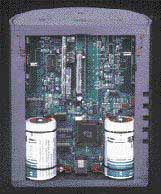 |
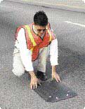
| Photo 1. Groundhog permanent traffic counters mounted in holes in pavement report cars detected by GMR sensors back to a central data collection point using spread-spectrum technology. |
Vehicle Detection. In applications involving the detection of motor vehicles (see Photo 1), the Earth's magnetic field acts as a biasing magnet, resulting in a magnetic signature from various parts of the automobile as it passes the sensor. The X, Y, and Z components of the signature can be detected by magnetic sensors buried in the road or placed on the side of the road (see Photos 2 and 3). Figure 9 shows the three components for a small automobile. The X direction is the direction of travel, and the Z component is vertical. The presence of a stationary vehicle can be detected by a single sensor. Measured at the surface of the road, the magnetic field from an automobile is similar in size to the Earth's magnetic field (i.e., about 1/2 Oe [40 A/m]). Therefore, the sensor and its circuitry must be nulled for this effect after they are installed.
Detection of stationary vehicles is important for traffic control at traffic lights and for monitoring parking spaces and resetting parking meters. Magnetic sensors can also be used to monitor moving traffic. In one such application, the sensors count and classify motor vehicles passing over portable or permanent sensors in the road. By using two sensors separated by a small distance, speed and vehicle length can be calculated for traffic classification. Small, low-powered GMR sensors let manufacturers package the sensors, electronics, memory, and battery in a low-profile protective aluminum housing the size of your hand [12]. Similarly, circuits with two sensors can monitor the presence and speed of trains approaching road crossings, making it possible to lower the crossing gates at an appropriate time.
Eddy Current Detection. These methods are used not only in proximity sensors but also in nondestructive evaluation of conducting metals. Applying magnetic sensors to eddy current sensing is similar to back biasing a magnetic sensor. A coil applies an AC field to the material under test. The coil is oriented so that its magnetic field is not in the same direction as the sensitive axis of the magnetic sensor and will not affect the sensor.
 |
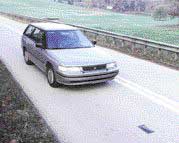
| Photo 2. HighStar traffic classifiers in their protective rubber enclosures are easily placed and removed on roads because of the lack of connection wires. |
 |
| Photo 3. Two GMR sensors in this nuMetrics HiStar traffic classifier record the length of the car into one of several bins for highway use studies. (Photos courtesy of nuMetrics, Uniontown, PA.) |
 |
| Figure 9. A 3-axis magnetic field sensor records the signature in 3D of an automobile passing in the X direction. Information from two sensors separated along the X direction can measure the speed and length of the vehicle. The maximum field recorded is 33 A/m (500 mOe). |
Eddy currents generated by the applied AC field in a continuous conducting sheet below the sensor create a mirror image of the field from the coil and do not affect the magnetic sensor. An imperfection or crack in the conductor will change the symmetry of the eddy currents, resulting in a component of the magnetic field along the sensitive axis of the magnetic sensor.
Eddy currents shield the interior of the conducting material with the skin depth related to the conductivity and the frequency. By changing frequency, different depths of the material can be probed. GMR sensors, with their wide frequency response (from DC to the multimegahertz range), are well suited to this application. The small size of a GMR sensing element increases the resolution of defect location as the detector is scanned over the surface in two dimensions [13]. For 1D scans, an array of detectors can be used. Figure 10 shows the configuration of the sensor and coil for eddy current detection.
Geophysical Surveys. This category of surveying increasingly relies on magnetic sensors. Airborne surveys of magnetic anomalies are used to locate bodies of magnetic ore, which have magnetic fields considerably less than that of the Earth's. If the magnetic surveys are conducted on the ground, the survey teams must use portable equipment. Low-field GMR sensors are well suited for these applications because of their sensitivity and the ease with which they can be packed into remote areas.
Engineers using eddy currents and magnetic sensors can detect changes in the conductivity of soil caused by the presence of water. Using the same technology, you can also locate conducting pipes and nonconducting pipes containing water.
To perform eddy current detection, you don't have to place electrodes in the ground, pass currents through the ground, or measure potentials. The wide bandwidth of GMR sensors lets you perform both time and frequency domain measurements simultaneously. Arrays of sensors make 2D and 3D imaging possible.
Studies have shown that liquid organic compounds react with clays with varying response times to a given stimulus. Therefore, with a large bandwidth, it may be possible to not only detect subsurface water flow but also determine organic contaminants.
Biomedical Sensing. The sensing of body position plays a role in various medical evaluations (e.g., the tracking of the movements of the eye or a limb). Position data can be correlated with other information, such as electromyogram (EMG) readings, to diagnose movement disorders. In some cases, a small magnet can be attached to the body part being monitored. For example, small magnets can be placed in scleral contact lenses. The position of the magnet can then be monitored by magnetic sensors mounted on an eyeglass frame.
A 3D measurement of the motion of a limb--including vertical inclination and horizontal azimuth--has been accomplished using three accelerometers and three orthogonal GMR sensors measuring vector components of the Earth's magnetic field [7].The system is small enough for long-term ambulatory measurements of patients during normal activities. Three magnetic sensors are required because the Earth's field is a vector with horizontal and vertical components. By measuring all three components of the field, the orientation of the triaxial sensor relative to the fixed direction of the Earth's field can be calculated. The calculation is similar to that used with magnetic sensors in compassing applications [1]. Care must be taken to bias the sensors onto a portion of their operating curve that will ensure that rotating the sensor in the Earth's field will not result in passing a minimum in the response curve (see Figure 6).
A proof-of-concept biosensor experiment has shown the value of using GMR sensors with magnetic microbeads in a Bead Array Counter (BARC) [8]. An array of 80 mm by 5 mm GMR sensor elements was fabricated from sandwich GMR material. Each sensor was coated with biological molecules that bond to various materials being assayed.
The magnetic microbeads are also coated with the materials to be analyzed. The microbeads in suspension settle on the GMR sensor array, where specific beads bond to specific sensors only if the materials are designed to attract each other. Nonbinding beads can be removed by a small magnetic field. The beads are then magnetized at 200 Hz by an AC electromagnet. The 1 µm microbeads are made up of iron oxide particles, which have little or no magnetization in the absence of an applied field. A lock-in amplifier extracts the signal at twice the exciting frequency from a Wheatstone bridge constructed of two GMR sensor elements (one of which is used as a reference) and two normal resistors. High-pass filters eliminate offset and the necessity of balancing the two GMR sensor elements.
 |
| Figure 10. Eddy current detection of defects in conducting sheets uses an AC magnetic field generated by a drive coil and a magnetic sensor. The coil positioned around the sensor produces no magnetic field along the sensitive axis of the thin film GMR sensor in the absence of a defect. The side and top views of the arrangement of coil and sensor are shown. |
With this detection system, the presence of as few as one microbead can be detected. The miniature nature of GMR sensor elements lets an array simultaneously test for multiple biological molecules of interest.
Summary
GMR magnetic field sensors are making their way into many low-field applications, from counting automobiles to detecting micrometer-sized beads in bioassay. Their small size, low power requirements, and low cost make them attractive in applications requiring arrays of sensors.
Commercially available GMR sensors are sensitive enough to verify currency over gaps of several millimeters and classify vehicles several meters away. The new GMR technology, SDT, promises to extend low-field solid-state sensing into areas previously dominated by larger, power-hungry devices.
The array of products using small fields or small field changes will expand significantly and alter the way traditionally difficult measurements are reliably made. The advances will take time and resources to perfect, but gradual changes will soon become apparent in products that are now under development. Magnetic sensing technology is moving forward, sensing smaller and smaller fields.
References
1. Michael J. Caruso et al. Dec. 1998. "A New Perspective on Magnetic Field Sensing," Sensors, Vol. 15, No. 12:34-46.
7. B. Kemp et al. 1998. "Body Position Can Be Monitored in 3D Using Miniature Accelerometers and Earth-Magnetic Field Sensors," Electroencephalography and Neurophysiology, Vol. 109:484-488.
8. D.R. Baselt et al. 1998. "A Biosensor Based on Magnetoresistance Technology," Biosensors & Bioelectronics, Vol 13:731-739.
10. Jacob Fraden, AIP Handbook of Modern Sensors: Physics Designs and Applications (American Institute of Physics, New York, 1993), pp. 243-262.
11.H. T. Hardner et al. "Fluctuation-dissipation relations for giant magnetoresistive 1/f noise," Phys. Rev. B, Vol. 48, No. 21:16 156-16 59.
12. "Tiny Sensor Measures Vehicle's Speed," nu-metrics News Release, 1998. www.nu-metrics.com
13.T. Dogaru and S. T. Smith. "A GMR-Based Eddy Current Sensor" (to be published in IEEE Trans Magn).