
Extracting useful knowledge from raw sensor data is not a trivial task. Conventional data analysis tools might not be suitable for handling the massive quantity, high dimensionality, and distributed nature of the data. Recent years have seen growing interest in applying data mining techniques to efficiently process large volumes of sensor data [1].
 |
Data mining, a critical component of the knowledge discovery process (Figure 1), consists of a collection of automated and semi-automated techniques for modeling relationships and uncovering hidden patterns in large data repositories [2, 3]. It draws upon ideas from diverse disciplines such as statistics, machine learning, pattern recognition, database systems, information theory, and artificial intelligence.
 Figure 1. The overall process of knowledge discovery from data (KDD) includes data preprocessing, data mining, and postprocessing of the data mining results |
Data mining has been successfully used on sensor data in applications as diverse as human activity monitoring [4], vehicle monitoring [5], and vibration analysis [6]. This article presents an overview of such techniques and describes some of the technical challenges that must be overcome when mining sensor data.
Preprocessing Steps
Before data mining techniques can be applied, the raw data must undergo a series of preprocessing steps to convert them into an appropriate format for subsequent processing. The typical preprocessing steps include:
- 1. Feature extraction—to identify relevant attributes for a data mining task using techniques such as event detection, feature selection, and feature transformation (including normalization and application of Fourier or wavelet transforms)
- 2. Data cleaning—to resolve data quality issues such as noise, outliers, missing values, and miscalibration errors
- 3. Data reduction—to improve the processing time or reduce the variability in data by means of techniques such as statistical sampling and data aggregation
- 4. Dimension reduction—to reduce the number of features presented to a data mining algorithm; principal component analysis (PCA), ISOMAP, and locally linear embedding (LLE) are some examples of linear and nonlinear dimension reduction techniques
Data mining can be broadly classified into four distinct tasks, which will be discussed in the next four sections.
Predictive Modeling
The goal of predictive modeling is to build a model that can be used to predict—based on known examples collected in the past—future values of a target attribute. There are many predictive modeling methods available, including tree-based, rule-based, nearest neighbor, logistic regression, artificial neural networks, graphical methods, and support vector machines [2]. These methods are designed to solve two types of predictive modeling tasks: classification and regression. Classification deals with discrete-valued target attributes; regression, with continuous-valued target attributes. For example, detecting whether a product on the assembly line is good or defective is considered a classification task, while predicting the amount of rainfall in summer is a regression task.
An example of classification is illustrated by the 2D data in Figure 2 (page 15). Let each data point represent measurements taken by temperature and vibration sensors attached to the engine of a vehicle. Data points shown as crosses are measurements taken when the engine is operating under normal conditions and the squares are conditions prior to engine breakdown. A classifier can be trained to predict whether an engine will operate normally or will labor. Training a classifier means learning the decision boundary that separates measurements that belong to the different classes. Thus, any measurements that fall within the boundaries in Figure 2 will be classified as normal and those outside will signify abnormal conditions.
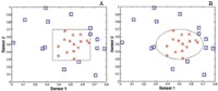 Figure 2. Classification of a 2D data set using (A) support vector machine and (B) decision tree classifiers; dashed line represents decision boundary for separating examples from two different classes (squares and crosses) |
Note that each classification technique has its own way of representing the shape and learning the location of the decision boundary. Some techniques (e.g., artificial neural networks and nearest neighbor classifiers) can produce very flexible boundaries, allowing them to model any type of classification problems. Others may produce more rigid boundaries, e.g., the hyper-rectangles created by decision tree classifiers. There are also techniques that can get a little overzealous—trying to fit all the previously observed examples (including noise)—which leads to a common pitfall known as overfitting. Care must be exercised to ensure that the classification technique chosen produces the desired boundary without overfitting the training data.
Cluster Analysis
Cluster analysis seeks to divide a data set into several groups so that data points belonging to the same group are more similar to one another than they are to those in a different group. Some of the techniques commonly used for clustering include k-means, self-organized maps, Gaussian mixture models, hierarchical clustering, subspace clustering, graph-based algorithms (e.g., Chameleon and spectral clustering), and density-based algorithms (e.g., Denclue and DBScan) [2].
The differences among these techniques lie in how the distance between data points is computed and how the cluster membership of a data point is determined. K-means uses the Euclidean distance as the underlying measure and places a data point into the cluster that has the shortest distance from its center. Figure 3 illustrates the results of applying k-means clustering to measurements from the Earth Science domain. Each location on the map is characterized by its climate and terrestrial features such as temperature, precipitation, soil moisture, and vegetation types. Using cluster analysis, scientists can identify regions that exhibit similar features in terms of their climate and terrestrial patterns.
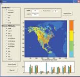 Figure 3. An example of k-means clustering on Earth Science data |
Association Analysis
Association analysis aims to discover strong co-occurrence relationships among events extracted from data. The discovered relationships are encoded in the form of logical rules. For example, the following rule, generated from sensor data collected by a wearable body-monitoring device, indicates the typical sensor readings of a sleeping person:
(heat flux Ε [4.48, 12.63] AND accelerometer Ε [0.86, 1.04]) _ Action = Sleep (accuracy = 99.94%)
Figure 4 (page 15) shows the distribution of heat-flux and accelerometer measurements when the person is sleeping (in red) or when performing other activities (in blue). Notice that the preceding rule summarizes one of the dense regions of red points into a logical description that can be easily interpreted by domain experts. Although the rule does not cover all sleeping cases, its accuracy is very high (>99%). There are many other rules—covering the remaining regions of the feature space—returned by the association analysis algorithm, but for present purposes only one of these rules is explored here.
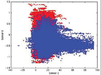 Figure 4. Distribution of heat-flux and accelerometer readings for a human subject; red points correspond to measurements taken when subject is sleeping and blue points correspond to those captured when subject performs other activities |
Association analysis has been extended to discover more complex structures, such as sequential and subgraph patterns. For example, a sequential pattern discovery algorithm has recently been developed to mine event logs generated from the assembly lines of manufacturing plants at General Motors [7]. Using this approach, interesting patterns relating the different status codes of an assembly line are derived. The information can be used to help improve the throughput of a line.
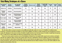 Data Mining Techniques at a Glance |
Anomaly Detection
Anomaly detection, also known as outlier or deviation detection, seeks to identify instances of unusual activities present in the data. A common way to do this is to construct a profile of the normal behavior of the data (Figure 5) and use it to compute the anomaly scores of other observations. Among the widely used anomaly detection techniques are statistical-based approaches such as Grubbs test and boxplots, and distance-based, density-based, and cluster-based techniques. In the distance-based approach, the normal profile corresponds to the average distance between every observation to its corresponding kth closest neighbor. If the distance from a given observation to its kth closest neighbor is significantly higher than the overall average, then the observation may be regarded as an anomaly.
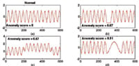 Figure 5. Detection of anomalies from time series segments; time series on upper left corner diagram is normal, while the rest contain anomalies of some type |
The key challenge of an anomaly detection algorithm is to maintain a high detection rate while keeping the false alarm rate low. This requires the construction of an accurate and representative normal profile, a task that can be very difficult for large-scale sensor network applications.
Consider This
There are several issues we must consider when applying data mining techniques to sensor data. First, we need to determine the appropriate computational model. There are two general models of computation: centralized and distributed (peer-to-peer) [8]. In the centralized model, each sensor transmits the data it has collected to a central server, which fuses the sensor readings and performs extensive analysis on the aggregated data. An obvious drawback of this approach is its high consumption of energy and bandwidth. Furthermore, it is not scalable to very large numbers of sensors. The distributed model, on the other hand, requires each sensor to perform some local computations before communicating their partial results to other nodes in order to obtain a global solution. This approach is more promising, but it requires every sensor to have an onboard processor with a reasonable amount of memory storage and computing power.
Sensor data characteristics present additional challenges to the data mining algorithm. These data tend to be noisy or to contain measurements with large degrees of uncertainty. Probability-based algorithms offer a more robust approach for handling such problems. Another issue to consider is missing values due to malfunctioning sensors. This problem can be addressed in many ways, either during preprocessing or during the mining step itself, e.g., by discarding the observations or estimating their true values based on the distribution of the remaining data. The massive streams of sensor data generated in some applications make it impossible to use algorithms that must store the entire data into main memory. Online algorithms provide an attractive alternative to conventional batch algorithms for handling such large data sets. Finally, the data mining algorithm must consider the effect of concept drift, where characteristics of the monitored process may change over time and render the old models outdated. This problem can be addressed using a mechanism that helps the model to "forget" its previous information.
In short, data mining provides a suite of automated tools to help scientists and engineers uncover useful information hidden in large quantities of sensor data. It also provides an opportunity for data mining researchers to develop more advanced methods for handling some of the issues specific to sensor data. For a list of the many commercial and publicly available data mining software packages available, see www.kdnuggets.com/software/index.html.
References
1. Proc 1st Intl Workshop on Data Mining in Sensor Networks, www.siam.org/meetings/sdm05/sdm-sensor-networks.zip, 2005.
2. P-N Tan, M. Steinback, and V. Kumar, Introduction to Data Mining, Addison-Wesley, 2005.
3. J. Han and M. Kamber, Data Mining: Concepts and Techniques, Morgan Kaufmann, 2000.
4. M. Perkowitz et al., "Mining models of human activities from the Web," Proc 13th Intl Conf on World Wide Web, New York, NY, May 2004.
5. Agnik, LLC, Mine Fleet: A Vehicle Data Stream Mining System, www.agnik.com/vehicle.html.
6. K. McGarry and J. MacIntyre, "Data mining in a vibration analysis domain by extracting symbolic rules from RBF neural networks," Proc 14th Intl Congress on Condition Monitoring and Engineering Management, Manchester, U.K., Sept. 2001.
7. S. Laxman, P.S. Sastry, and K.P. Unnikrishnan, "Discovering frequent episodes and learning hidden Markov models: a formal connection," IEEE Transactions on Knowledge and Data Engineering, Vol. 17, No. 11, 2005, pp. 1505–1517.
8. I.F. Akyldiz et al., "A survey on Sensor Networks," IEEE Communications Magazine, Vol 40, 2002, pp. 102–114.
Pang-Ning Tan, PhD, can be reached at Michigan State University, Dept. of Computer Science and Engineering, East Lansing, MI; 517-432-9240, [email protected].