An Introduction to Analog Filters

Hundreds if not thousands of different kinds of filters have been developed to meet the needs of various applications. Despite this variety, many filters can be described by a few common characteristics. The first of these is the frequency range of their pass band. A filter's pass band is the range of frequencies over which it will pass an incoming signal. Signal frequencies lying outside the pass band are attenuated. Many filters fall into one of the following response categories, based on the overall shape of their pass band.

Low-pass filters pass low-frequency signals while blocking high-frequency signals. The pass band ranges from DC (0 Hz) to a corner frequency F_C.

High-pass filters pass high-frequency signals while blocking DC and low-frequency signals. The pass band ranges from a corner frequency (F_C) to infinity.

Band-pass filters pass only signals between two given frequencies, blocking lower and higher signals. The pass band lies between two frequencies, F_L and F_H. Signals between DC and F_L are blocked, as are signals from F_H to infinity. The pass band of these filters is often characterized as having a bandwidth that is symmetric around a center frequency.

Band-stop filters block signals occurring between two given frequencies, F_L and F_H. The pass band is split into a low side (DC to F_L) and a high side (F_H to infinity). For this reason, it's often simpler to specify a band-stop filter by the width and center frequency of its stop band. Band-stop filters are also called notch filters, especially when the stop band is narrow.

Figure 1 shows how each of these filters operates on a swept-frequency input signal.

 

 

In the examples, the signal increases continuously in frequency, from a low frequency to a high frequency. When the signal frequency is within the filter's pass band, the filter passes the signal. As the signal moves out of the pass band, the filter begins to attenuate the signal.

Note that the transition from the pass band to the stop band is a gradual process, where the filter's response decreases continuously. Although you can make this transition arbitrarily sharp (at the cost of filter complexity), it can never be instantaneous, at least not in filters physically realizable with today's technology.

The Bode and Phase Plots

Bode plots describe the behavior of a filter by relating the magnitude of the filter's response (gain) to its frequency. An example of this type of plot is shown in Figure 2.

 

 

The key feature of this graph is that both axes have logarithmic scales. The horizontal ax[s represents frequency, measured in hertz, and the vertical axis is measured in decibels.

Decibels are a logarithmic measure of power, where an increase of 10 dB represents a 10-fold increase in power. Because power in an electrical signal is related to the square of voltage, a factor of 10 increase in the voltage of a signal is represented by an increment of 20 dB. The advantage of drawing a filter's response curve on a Bode plot is that it provides an easy way to describe the filter's response over several decades of frequency and several orders of magnitude. The decibels of gain of a filter relate to the ratio between input and output voltages:

(1)

The low-pass response curve in Figure 2 also illustrates a few characteristics common to many types of filters.

Corner Frequency. Because a real filter rolls off gradually, you usually specify the corner frequency as the frequency at which the response is 1/2 (0.707) of that in the pass band. Because electronic engineers traditionally describe relative signal strengths in decibels, the frequency is also referred to as the –3 dB point.

Attenuation Rate. The transition between the pass band and the stop band is a continuous function, and the rate at which this transition occurs is a common metric used to select a filter. You commonly express the attenuation rate in decibels per decade, where a decade is a factor of 10 in frequency.

A high attenuation rate helps a filter distinguish between signals of similar frequency and is usually a desirable feature. The attenuation rate is also related to the order of a filter. For a low-pass or a high-pass filter, the attenuation rate will be –20 times the filter's order, in dB/decade. For example, a first-order filter will have an attenuation rate of –20 dB/decade, while a fourth-order filter will have an attenuation rate approaching –80 dB/decade.

Pass-Band Ripple. For many types of filters, the response does not decrease monotonically as frequency moves from the center of the pass band out toward the stop band. The magnitude of the response may vary inside the pass band, and this variation is called the pass-band ripple. Again, this metric is also specified in decibels. Pass-band ripple causes the frequency components of a signal to be amplified to different degrees. This has the effect of distorting the waveform of a signal passing through the filter.

In addition to affecting the amplitude of a signal, a filter can also cause changes in the phase of signal components. Figure 3 shows the amplitude and phase responses of a simple low-pass filter.

 

 

If you run sinusoidal signals of different frequencies through this filter, not only does the filter attenuate the higher frequency

Figure 4. A resistive voltage divider can serve as a starting point for understanding simple filters. The voltage appearing at the output is a fixed fraction of the voltage applied to the input. The ratio between Vout and Vin, or the gain, is determined by the values of RA and RB.

signals, but it also shifts their phase.

Note that the phase-shift plot describes the shift of sinusoidal signals. A filter's phase response is also important in the case of nonsinusoidal signals because phase shifts distort the waveforms. This is because nonsinusoidal signals can be viewed as combinations of sinusoidal signals of varying frequencies. Shifting the phase of these components relative to one another will change the shape of the overall waveform.

Filter Circuits 101

Although the design of filter circuits can require sophisticated analysis, you can develop an understanding of the basic concepts with a minimum of math and circuit theory. As a starting point, consider the resistive voltage divider that is shown in Figure 4. The circuit provides an output voltage that is a fixed fraction of the input voltage. The relationship between the input and output voltages is given by:

(2)

Because a resistor's characteristics (in the ideal case) don't vary as a function of frequency, the relationship is valid for both DC and AC signals. If the values of the resistors are frequency dependent, however, the ratio of output to input voltage will also become frequency dependent.

If you consider an AC resistance to be the ratio between the voltage across a component and the current through it, then inductors and capacitors exhibit resistances dependent on the frequency of the applied signal. There is a significant difference, however, between the resistance of a resistor and that of an inductor or a capacitor. For sinusoidal signals, voltage and current waveforms are always in phase in a resistor.

In the cases of capacitors and inductors, the current is 90° out of phase with the voltage. The difference is expressed by referring to the resistance of the latter devices as imaginary, and they are represented by using imaginary numbers (j). The term impedance denotes resistances that have imaginary components. For AC signals of frequency f, the complex impedances of resistors (Z_R), capacitors (Z_C), and inductors (Z_L) are given by:

(3)

While a resistor has a constant impedance over frequency, the impedance of a capacitor decreases with increasing frequency while that of an inductor increases.

With the tool of complex impedance, you can analyze the behavior of simple filters based on voltage divider circuits. Consider the circuit shown in Figure 5A, in which a capacitor has been substituted for the lower resistor in a voltage divider.

 

 

As the input signal's frequency increases, the impedance of the capacitor will decrease, resulting in less output signal. By substituting the capacitor's complex impedance for R_B, you can express the output voltage in the following way:

(4)

From Equation 4, you can see that at zero frequency (DC) the ratio of output to input is 1, and it decreases as frequency increases. Complex output voltage, however, isn't any more intuitive than complex impedance. By taking the magnitude of Equation 4 (see the sidebar "They Don't Call It Complex Math for Nothing"), you get a relationship that describes the ratio between the magnitudes of the input and output for sinusoidal signals:

(5)

When you set f = 1/2RC, the response is 1/2, or –3 dB from that of DC. Another feature of this filter is the attenuation rate. As frequency increases above the –3 dB frequency, the response becomes inversely proportional to the frequency. The response decreases a factor of 10 for every factor of 10 increase in frequency, yielding an attenuation rate of –20 dB/decade. Similar analysis can be made for various other simple filters based on voltage division. A low-pass filter based on an inductor is shown in Figure 5B, and two high-pass filters a.e shown in Figures 5D and 5E.

Op Amp Filter Circuits

You can perform similar analysis on simple circuits based on implementations other than the voltage divider. For example, another circuit of general interest is a closed-loop amplifier built around an operational amplifier (op amp). This circuit (see Figure 6A) provides a gain of –R_f/R_i, assuming an ideal op amp with infinite gain.

 

 

If you replace the feedback resistor R_f with a capacitor C, as shown in Figure 6B, the resulting gain vs. frequency is:

(6)

The gain for this circuit, like that of the low-pass filter, is inversely proportional to frequency, but it differs in that it increases to infinity for DC signals. Also, because the gain is imaginary, there is always a 90° phase difference between the input and the output (i.e., the circuit will always convert a cos(x) input into a sin(x) output). From a time-domain standpoint, the circuit integrates its input, and for this reason, it is called an integrator.

Replacing the input resistor (Ri) of our original op amp with a capacitor results in a circuit with a response proportional to increasing frequency (see Figure 6D). This circuit takes the derivative vs. time of the input signal, and for this reason, it's called a differentiator.

Figure 7. One advantage of an active filter is that in addition to filtering a signal it can also amplify it. This circuit provides a DC gain of -R2/R1 and a corner frequency of 1/2R2C.

While there are a number of applications in which the straight-line Bode plots of the integrator and differentiator are useful, you can create more interesting filter circuits using series-parallel networks of resistors and capacitors around the op amp. One simple example of such a network is shown in Figure 7. This circuit implements a low-pass filter.

Although this filter uses more components than a simple RC filter, it lets you amplify and filter a signal in one signal-processing stage. Perhaps more importantly, because the output impedance of the op amp is low, you can cascade filter stages without having to worry much about loading effects. With the filter circuits first presented, which don't use op amps, any significant load on the output of the filter could change its frequency response and gain. Filters that contain amplifier circuits, such as the one presented in this section, are called active filters.

Combining Simple Filters

Because you can readily cascade the active filters just described, you can easily predict the behavior of combinations of these filters and use them as building blocks to construct more complex circuits. Two of the simpler combinations are series connections and parallel connections. A series connection of two filters with transfer functions g(f) and h(f) results in an overall transfer function of g(f) × h(f). In a parallel connection, the outputs of the filters are summed, and the filter functions add g(f) + h(f).

By linking low-pass and high-pass filters via a series connection, you can create a band-pass filter if the corner frequency of the low-pass device is greater than that of the high-pass device (see Figure 9A).

 

 

And you can use the parallel connection to make a band-stop, or notch, filter if the corner frequency of the low-pass filter is lower than that of the high-pass filter (see Figure 9B). Other arrangements based on series and parallel configurations can be used to develop additional filters with more complex characteristics.

One obvious series combination is that of cascading identical low-pass or high-pass sections to get a filter with a steeper attenuation rate. For example, you would expect that cascading two low-pass filters with –20 dB/decade attenuation rates would result in one with a

Figure 11. Circuits containing both capacitors and inductors often exhibit resonance, a phenomenon that when properly used lets you make filters with sharp transitions between their pass band and stop band.

–40 dB/decade attenuation rate. While the ultimate attenuation rate will indeed approach –40 dB/ decade, the sharpness of the filter's "knee" will decrease. This makes it difficult to build a more selective filter by simply cascading identical sections.

Resonant Circuits

What if you replace both resistors in a voltage divider with capacitors and inductors? If you use either just capacitors or just inductors, the imaginary components cancel out, and the circuit behaves much like a resistive voltage divider, at least for AC signals. If you use a capacitor for one leg and an inductor for the other (see Figure 11A), new behavior emerges. If you substitute the imaginary impedances into the voltage divider equation, you obtain:

(14)

The response of this circuit is completely real—meaning there's no phase shift between input and output. It's also a low-pass filter because the response is unity (1) at DC and drops to zero as frequency is increased. If you set f = 1/2LC, however, the denominator of the response equation goes to zero, implying that you get infinite output voltage for a finite input voltage. Although an actual circuit wouldn't produce an infinite output voltage, the peak can still be quite high, with a maximal response occurring when f = 1/2LC. This frequency is called the circuit's resonant frequency.

Resonance is a phenomenon that is qualitatively different from that which can be obtained in a passive filter circuit consisting of only resistors and capacitors. If you plot the LC circuit's time-domain response to a step input, you see that it oscillates, or rings. Resonance results because electrical energy is periodically transferred back and forth between two or more circuit elements—the inductor and the capacitor in the above case. Energy in a passive RC or RL circuit, however, only flows in one direction as the circuit moves toward a steady state. For this reason, these circuits don't oscillate.

One useful feature of LC filter circuits is that they have steeper attenuation rates (e.g., –40 dB/decade) than RC filters. This stems from the fact that the circuits have responses that vary at a rate of 1/f² instead of 1/f. While you can get this attenuation rate by cascading two RC filters, as discussed above, the LC circuit's resonant peak allows for a sharper "knee" at the frequency where the filter transitions from pass band to stop band. By inserting a resistor in series with the inductor, the magnitude of the response peak can be reduced, or damped, to control the sharpness of the knee. The degree of peaking in a resonant filter can be quantified by a measure known as the filter's Q. For the case of the RLC low-pass filter shown above, Q is given by:

(18)

With RLC filters, you can also get low-pass, high-pass, band-pass, and band-stop functions by rearranging the circuit elements. Figure 14 shows the circuit configuration for these filters.

 

 

Active Filters Revisited

RLC passive filters are widely used because many applications require filters with high attenuation rates and sharp knees. Unfortunately, you need one or more inductors to implement an RLC filter. Compared with resistors and capacitors, inductors tend to be large, expensive, and have poor tolerances. Additionally, because inductors generate magnetic fields, they can cause unwanted interference with other nearby components.

Figure 16. Active filters using just resistors and capacitors provide the benefits of resonance. The voltage-controlled voltage source (VCVS) topology readily provides both low-pass (A) and high-pass (B) filters.

Fortunately, you can build circuits that have resonance by using different circuit topologies consisting only of resistors, capacitors, and amplifiers. One such set of topologies is called voltage-controlled voltage source (VCVS) filters, of which low-pass and high-pass versions are shown in Figure 16.

Both these circuits provide filters with –40 dB/decade attenuation rates and sharper corners than a cascade of two first-order filters. In each, the op amp acts as a noninverting amplifier with a greater-than-unity gain. The gain of the amplifier is determined by (R₃ + R₄)/R₃.

From an intuitive standpoint, you can see that the circuit shown in Figure 16A has gain at DC and rolls off as the frequency increases. This circuit will behave as a low-pass filter. Similarly, because the circuit in Figure 16B has its capacitors in the signal path, it will have zero response at DC, and the response will increase as frequency increases.

Both the corner frequency and Q of each of these filters is determined by the values of the capacitors (C1 and C2), the resistors (R1 and R2), and the amplifier gain. For a filter with a maximally flat pass band and a corner frequency of 1/2RC, the amplifier gain should be set to 1.586, R₁ = R₂ =R, and C₁ = C₂ = C.

Figure 17. The Sallen and Key filter is a popular type of voltage-controlled voltage source (VCVS) filter that uses a unity-gain amplifier and provides a pass-band gain of unity while still providing a second-order response. A corresponding high-pass version can be made by exchanging the resistors and capacitors.

A disadvantage of the VCVS filters described here is that the pass-band gain is not necessarily equal to one. When unity pass-band gain is needed, you can wire the amplifier as a unity-gain follower. This circuit is called a Sallen and Key filter, and the low-pass case is shown in Figure 17. Assuming that R1 = R2 =R and C1 = C2 = C, the corner frequency of this particular filter is given by f = 1/2RC and the attenuation rate of the circuit will also approach –40 dB/decade.

Although the above examples are of relatively simple second-order filters, they can be used as building blocks to construct filters of higher order and sharper knees. The theory of how to specify and design these higher order filters, however, is far beyond the scope of this article.

SIDEBARS:

They Don't Call It Complex Math for Nothing Although such dynamic systems as filters are most naturally described with differential equations, this can make analysis difficult. By representing voltages, currents, and impedances with complex numbers, it's possible to analyze filters using only algebra. And though it requires a bit more bookkeeping than simple arithmetic, manipulating complex numbers is straightforward if you know the rules. First of all, a complex number is represented as the sum of a real number and an imaginary number, such as 23 + 5j. Adding and subtracting complex numbers is accomplished by separately adding the real and complex parts, as shown in the following examples: (3 + 6j) + (7 + 2j) = (3 + 7) + (6 + 2)j = 10 + 8j (2 + 4j) – (7 + 6j) = (2 – 7) + (4 – 6)j = –5 – 2j (7) Multiplying complex numbers is similar to multiplying polynominals. The real and complex components in each number to be multiplied must multiply those in the other number. Two important points to remember, however, are that multiplying an imaginary number by a real number results in an imaginary number, but the result of multiplying two imaginary numbers is a real number. Furthermore, because "j" is defined as -1, j x j = –1. The above considerations result in the following formula for multiplying complex numbers: (a + bj) × (c + dj) = (ac – bd) + (ad + bc)j (8) where: (ac-bd) = the real part of the result (ad+bc)j = the imaginary part of the result An example of complex multiplication is: (2 + 3j) × (4 + 5j) = (2 × 4 – 3 × 5) + (2 × 5 + 3 × 4)j = –7 + 22j (9) Dividing two complex numbers is, well, a bit more complex. Consider dividing the following complex numbers: (10) The first step in the division process is to multiply both the numerator and denominator of the expression by what is known as the complex conjugate of the denominator. The complex conjugate of a number has the same real value but a negated imaginary value. The complex conjugate of c + dj is therefore c – dj. Multiplying a complex number by its conjugate always results in a completely real result. Multiplying the denominator in this way results in a simple real number (c2 + d2) with which you can divide the real and imaginary parts of the numerator:   (11) Finally, because most test instruments are designed to measure real signals, you need a method of relating the complex results delivered by the math to the real voltages and currents measured on the bench. The two most important interpretations of a complex value are the signal's magnitude and phase. If you plot a complex number on the complex plane and draw a line from the origin to the point where that number lies, the magnitude is the length of that line, and the phase is simply the angle (q°) between that line and the positive real axis (see Figure 8).   Figure 8. The magnitude and phase of a complex number can be interpreted geometrically. The magnitude of a complex number is the length of the line connecting the number and the origin of the complex plane, and the phase is the angle between the line and the real axis.   To obtain the magnitude, you apply the Pythagorean theorem to the real and imaginary parts of a complex value. In this case, you don't want to square the "j" because it will flip the sign of the b2 term. Both a2 and b2 should always end up as positive quantities:   (12) Calculating the phase is a bit more complicated because the formula you use depends on the relative sign and magnitude of the real and imaginary parts of the complex value. Note that this formula returns the phase in degrees over a ±180° range. Positive phase can be interpreted as lagging phase, or as the angle that an output signal lags behind an input signal (assuming sinusoidal signals):   (13)

Implementing a Crossover Crossover filters combine matched high- and low-pass filters to separate low- and high-frequency signals and direct the signals to separate outputs. Manufacturers often use crossover networks in audio systems to direct the frequency components of audio signals to the appropriate driver (e.g., tweeter, woofer, and midrange) in a loudspeaker. Although there are many ways of implementing crossover filters, one interesting and nonintuitive method is to use a single, low-pass element, such as an integrator, as the starting point. Figure 10 shows a feedback loop with an amplifier acting as the feed-forward element and an op-amp integrator providing feedback.   Figure 10. Wrapping a feedback loop around an integrator results in both low-pass and high-pass filter functions.   For simple feedback loops, such as the one shown in Figure 10, the general relation between input (X) and output (Y) is given by:   (15) where: a = the gain of the feedforward path b = the gain of the feedback path In this case, a is constant (1) and b is the complex gain provided by an integrator (1/2fRCj). Substituting these expressions for a and b yields the following expression for gain at the Y output:   (16) This expression describes a first-order high-pass filter with a corner frequency FC = 2RC. You can also obtain a low-pass filter by simply taking the output at another point in the circuit. The output of the integrator (Z) represents the high-pass function appearing at output Y, multiplied by the gain of the integrator. The resulting relation between Z and X is given by:   (17) This is recognizable as the gain function for a low-pass filter with a corner frequency FC = 2RC. Note that both the high-pass and the low-pass corner frequencies match each other because they are both ultimately derived from the integrator's gain function. Although this circuit can be built from discrete components, it can also be implemented with a Lattice ispPAC10 programmable analog circuit (see Figure 12).   Figure 12. The Lattice ispPAC10 can directly implement the crossover filter using no external components.   This device provides adjustable corner frequencies and a single-component realization. The onchip programmable capacitor associated with OA2 can be used to set the filter crossover frequency over a range of roughly 10–200 kHz. The actual corner frequency for both filter functions will vary slightly from that calculated for a given capacitor value because of finite bandwidth in the other amplifiers used in this circuit. Another effect of finite bandwidth is that the high-pass response curve will begin to roll off around 500 kHz, in actuality being a band-pass filter with an adjustable lower limit (see Figure 13).   Figure 13. The crossover filter provides both high-pass and low-pass functions with the same -3 dB frequencies.

The Easy Way to Design a Biquad Biquadratic filters, or Biquads, are popular circuits for implementing second-order low-pass and band-pass filters. Although the math required to design one is straightforward, finding the appropriate combinations of component values to realize a given filter can often be a challenge, especially if you need to meet tight performance specifications. Lattice Semiconductor's PAC-Designer software can make this task simple (see Figure 15).     Figure 15. Lattice Semiconductor's PAC-Design lets you design, simulate, and implement active filters with a few mouse clicks. 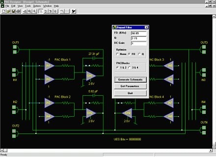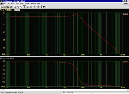By invoking the Biquad design macro, you can specify the corner frequency and the Q for a desired biquad, click a single button, and have an optimal design transferred into PAC-Designer's design screen. Simulation and validation of a proposed design can be performed in the PAC-Designer environment in a matter of seconds. When a suitable design has been determined, you can transfer it into silicon with one more mouse click. The total time required to go from a specification to working silicon can be less than five minutes.   Additional design macros provided with PAC-Designer also let you design, evaluate, and implement more complex, higher order filters in a similar manner.