|
Although the facility features many types of velocity measurement methods for operation under different test settings and environmental conditions, the inventory of sensor and transducer configurations can't always meet the novel requirements that arise. As a result, lab engineers have developed unique time-of-arrival velocity instrumentation based on break-paper, break-wire, photoelectric, inductance, photography, and photoexcitation techniques.
Recently, however, even these weren't enough to handle the lab's need for a benchmark technique of measuring velocity to determine the accuracy of the other measuring methods being used. Kaman Instrumentation Corp. provided the solution, not with an expensive new invention but instead by adapting a cost-effective off-the-shelf system.
The result, the Kaman KD-2300 dual-sensor velocity system, is used in the Impact Physics Lab's 0.50 caliber, light-gas-gun facility as a comparative standard to accurately measure projectile speeds over the entire velocity range. Using the KD-2300 as a standard, the Air Force can calibrate other devices used on the lab's higher velocity, higher caliber ranges, such as the powder, electro-thermal-chemical, and rail launcher facilities.
Theory
To understand the significance of the Kaman system, some background on projectile velocity testing is needed. The velocity of a launched projectile is calculated by dividing the base length, or the distance between two downrange measurement locations, by the difference of the times when the projectile arrives at these locations. Using the lab's existing sensors, engineers could record the time difference very accurately. During measurement, however, the distance between measurement locations could change. When break wires were used, for example, stretching before breaking caused the problem. When break papers were used, bulging before tearing was the culprit. Hence, the recorded data reflected the pretest position plus an increment that could not be measured. This led to an unknown error, because only the set position (measured between sensors) is used in the velocity calculation:
v = ds/dt
where:
s = space, t = time
The KD-2300 uses a 1 MHz carrier frequency to induce eddy currents in the projectile as it enters the oscillating electromagnetic field (EMF), typically 2 in. from the plane of the coil. Because the coils are open, the EMF extends in both directions, allowing 4 in. of engagement between the projectile and the coil field. The 1 MHz carrier frequency and the 4 in. engagement length allows the KD-2300 to detect the precise peak location of the projectile in relation to the coil regardless of projectile velocity. Therefore, the locus within the EMF where the projectile "triggers" a signal (the point used to determine the set distance between the sensors) is easily measured because the projectile can be manually positioned.
Using the Kaman instrument, engineers can precisely determine the times-of-arrival and the set distance. Consequently, the effective set distance of other time-of-arrival devices can be determined by comparison with the Kaman data. Using the value for velocity, v, from the Kaman sensor, and difference between times-of-arrival, dt, from the other devices being tested, the velocity calculation will provide the set distances.
Operation
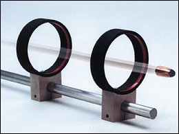
The Kaman system is dual coiled (see sidebar, "Adapting an Eddy Current Sensor") and consists of two standard sensor coils (Kaman part number 12CU), each mounted on a special open-coil form with a 2.5 in. dia. Each coil form is affixed to a standard pinch clamp and independently mounted onto a metal rod, allowing the user to easily adjust the distance between the coils by simply sliding them closer together or farther apart. The frequency response of the system at 50 kHz permits sensing of very high speed projectiles, far in excess of the 3000 fps specification.
System operation is simple. As the projectile approaches the first coil, eddy currents are induced and the voltage output—positive on the first coil—begins to increase. As the bullet reaches dead center of the first coil, the voltage output peaks to its highest level. As the projectile leaves the first coil, the voltage output decreases. As the projectile approaches the second coil, the same sequence occurs, except that the voltage output is negative.
Voltage output changes from both sensors are captured on an oscilloscope or data acquisition system. By correlating the time between the two peaks in voltage and the known distance (set position) between the coils, the velocity of the projectile is determined.
Benefits
Kaman's system has several benefits:
- Accurate peak voltage at the coil is independent of the actual location of the projectile when it reaches the coil. For instance, if the projectile is off to the left or right or up or down, accuracy is not affected. Lasers, for example, would require precise positioning of the projectile.
- Both coils are attached to the same output, so only one data acquisition input channel is required. This greatly simplifies the system in terms of fewer parts and also makes voltage peak comparisons easier, as they are contained on one output device.
- The system can be calibrated on site for various projectile materials, including steel, tungsten, lead, and aluminum.
- Calibration is as simple as centering the projectile within the sensor and adjusting the gain to 1 V.
- The system is low cost. Only one data acquisition system input is required, which can be any device with analog DC input.
- Delivery time is quick. Kaman can deliver the KD-2300 system in under six weeks because it was simply adapted from an existing off-the-shelf system.
Summary
The velocity measurement could have been made by using two single-coil systems. With two outputs, however, the user would be required to use two data acquisition inputs. Kaman was able to make the measurement with a single analog output and data acquisition input by a simple modification to a standard inductive bridge system. A general advantage of inductive bridge systems is their ability to be easily modified and adapted to application-specific systems.
SIDEBAR:
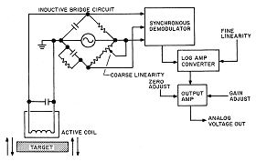
| Adapting an Eddy Current Sensor Typical inductive bridge systems use a single-coil sensor to generate eddy currents in the surface of a conductive target, as shown in Figure
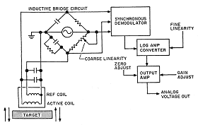
In a Kaman standard KD-2300 dual-coil system (see Figure 2), a reference coil is housed in the sensor and wired to the opposite side of the bridge from the active coil. This causes the thermal sensitivity spec to dramaticallyimprove because both legs of the balanced bridge are being affected equally by temperature-induced changes in the electrical properties of the coil.
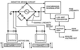
Figure 3 shows the modification that Kaman made to the dual-coil setup to enable the system to measure velocity. Here, the reference coil is separated from the active coil and becomes an active coil itself. As the target passesthe first coil, the bridge imbalance causes the output to swing positive. As the target passes the second coil, the output swings negative.
|