

Benefits Of Using An Inductance-to-Digital Converter For Linear Position Sensing
Accurate measurement of the linear position is a common challenge for many system designers whether it be automotive, industrial, or consumer markets. Example applications include determining car seat position, measuring the force applied to a brake or accelerator pedal, or measuring the position of a dimmer light switch or thermostat switch.
Many technologies cannot operate in the presence of oil, dirt, dust and moisture, or struggle with long-term reliability. Inductive sensing applies to these types of applications because it is a contactless and magnet-free technology that facilitates systems with very high measurement accuracy. It is insensitive to non-conductive environmental contaminants and offers high reliability at a low system cost.
An inductance-to-digital converter (LDC) measures inductance change that a conductive target causes when it moves into the inductor's AC magnetic field. The LDC measures this inductance shift to provide information about the position of the target over a sensor coil. The inductance shift is caused by eddy currents generated in the target due to the sensor's magnetic field. These eddy currents generate a secondary magnetic field that opposes the sensor field, causing a shift in the observed inductance. This can be used for precise positioning of the target as it moves laterally over the sensor coil.
In this article, we explore how to shape the AC-magnetic field of a PCB-routed inductor to utilize it for linear position sensing (see fig. 1). When compared to other linear position sensing technologies, inductive sensing provides the advantage that the size of the moving target is not related to the desired travel length. Therefore, a target that is significantly smaller than the required travel range can be used with this approach, enabling the advantages of inductive sensing in space-constrained applications.
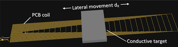
Fig. 1: Moving a conductive target laterally over a stretched PCB coil.
Concept
Two approaches to inductive sensing are available for linear position sensing. Both approaches work by changing coil inductance at different target positions:
- Use a circular coil and a shaped target, such as triangular
- Use a stretched coil and a rectangular target
Table 1 shows the key differences between these two approaches.
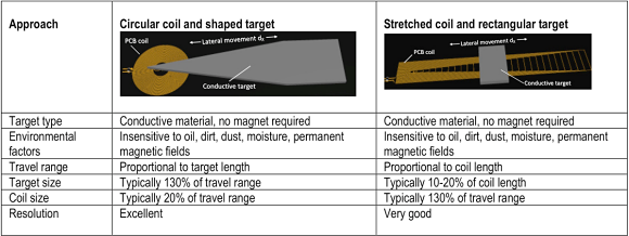
Table 1: Inductive sensing approaches for linear position sensing.
In contrast to shaping the target, it is possible to use a simple rectangular target and instead shape the AC-magnetic field. This can be achieved by 'stretching' a coil, such that it produces a stronger AC-magnetic field on one side versus the other. The coil in Figure 1 produces an AC-magnetic field that can be used to determine the position, dX, of a rectangular conductive target at a given target distance.
The highest density of magnetic field lines exists around the innermost turn, and the field line density decays towards the right side. Therefore, the peak strength of the AC-magnetic field lies left of the geometric center of the coil. Figure 2 shows a simulation of the magnetic field of a similar stretched coil design.
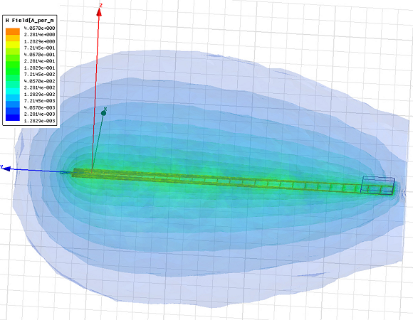
Fig. 2: This shows a magnetic field around a stretched coil.
Performance
Figure 3 shows an example of an inductor that generates a non-homogenous magnetic field. The inductor measures 100 mm x 15 mm, has 28 turns per layer on two layers, and has a 3.3 mm loop-stepping on one side. A 330 pF parallel capacitor is in parallel with the inductor to form the sensor, which is an L-C tank with a frequency of:
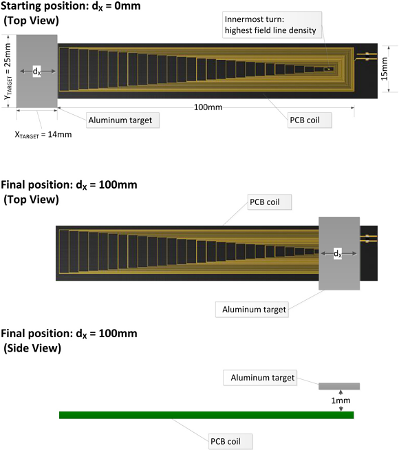
Fig. 3: Coil and target dimensions.
The target is a 1.5-mm thick, 14-mm x 25-mm piece of aluminum. However, other materials such a copper can be used. The size of the target is not as significant, as long as YTARGET ≥ the coil width and XTARGET covers several coil turns. Figure 3 shows the target position in the starting position (dX=0 mm) and the final position (dX=100 mm).
An example of an inductance-to-digital converter for precision linear position-sensing applications is the LDC1612 because the resolution of this 28-bit data converter provides measurement precision in the µm range. Its data output is a function of the sensor oscillation frequency and, therefore, of the coil inductance. Moving the aluminum target in Figure 3 (from dX=0 mm to dX=100 mm at a 1 mm target distance in 0.5 mm steps) and recording the data output results in the data output shown in figure 4.
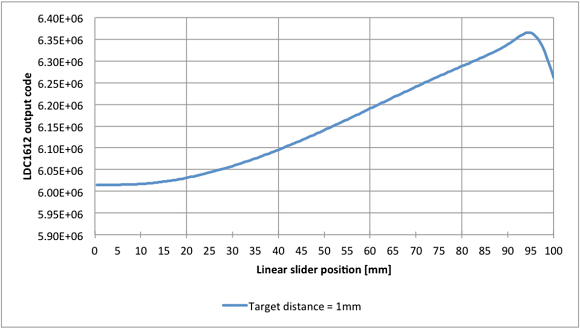
Fig. 4: Linear position versus an output code at a 1-mm target distance.
Maximum Useable Travel Range
The graph that results from sliding the target from dX=0 mm to dX=100 mm can be broken down into three distinct regions (see fig. 5): reduced resolution, optimal operating region, and unusable.
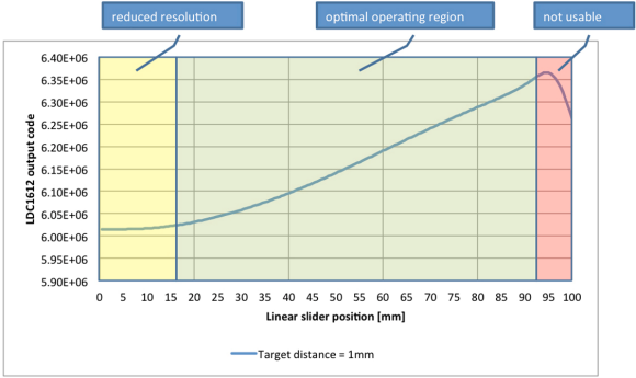
Fig. 5: Sliding the target from dX=0 mm to dX=100 mm identifies three regions.
Between 0.0 and 15 mm, the target enters the coil's magnetic field. This region can be used to determine target position, but its resolution is less than in the center region. For example, moving from dX=5.0 mm to dX=5.5 mm results in a frequency shift of 0.0026 percent, which creates a 77 code change in a 28-bit LDC. Therefore, the average code increase over this range is 0.15 codes per ?m. System accuracy requirements dictate whether or not this region can be used to determine linear position. High-precision applications may need to discard this region.
The optimal region for precision measurements is in the center region, which spans the sensor length from 15.0 mm to 92.0 mm. In this region, inductance decreases from 95.3 µH to 85.6 µH, which corresponds to a frequency shift of 11.35 percent. Inductance decrease over this range is mostly linear and can be used to determine target position to very high accuracy.
For example, the data shows that moving from dX=50.0 mm to dX=50.5 mm results in an output code change by 2,369 codes. This code change equates to an average increase of 0.21 µm/code. In this range, the LDC shows a maximum standard deviation of 0.69 µm, which is approximately equal to three codes. A 1 µm increment is approximately five codes, slightly more than the standard deviation, so the noise-free resolution is approximately nine codes, or about 2 µm.
Between dX=92.0 mm and dX=100.0 mm, the trend reverses. This reversal is due to the drop in magnetic field strength past the center coil loop. Since this region is non-monotonic, it is difficult to utilize for position-sensing.
Data shows that the usable travel range is less than the length of the coil, and also depends on system accuracy requirements. As a result, the coil design length needs to extend beyond the required travel range. As a rule of thumb, precision applications are possible with a coil size of 130 percent of the required travel distance. Applications with lower precision requirements may include a larger section of the reduced resolution region in Figure 5. Therefore, the coil length may be shortened to 120 percent or even 110 percent of the required travel distance.
The resolution can be further improved by using a longer target. The higher metal exposure of a longer target generates more eddy currents in the target, which cause a stronger opposing magnetic field. Therefore, if the target length XTARGET is extended, it will produce a higher frequency shift, and better resolution. However, a longer target also limits travel range and may not satisfy mechanical system constraints.
Target Distance
The magnetic field strength of the coil rapidly decays beyond one coil diameter distance. It is recommended to keep the target distance closer than one coil width. The coil in Figure 3 is suitable for target distances up to 15 mm. However, highest resolution is generally obtained when the target distance is kept as low as possible, as long as it complies with the LDC's device-specific boundary conditions. The highest inductance change, and hence the maximum resolution, occurs at the lowest target distance. Table 2 shows the inductance change at three different target distances.
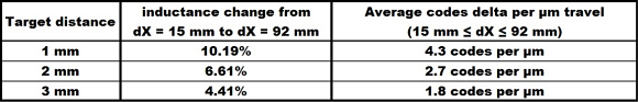
Table 2: Resolution at different target distances.
Given that the target distance has a different impact on the system inductance, it is necessary to ensure that any error introduced by the mechanical tolerance of the target distance does not exceed resolution requirements. In systems where linear position must be determined more accurately than tolerances in target height would normally allow, a dual-coil system can be used to compensate for the z-axis tolerance.
Such a system utilizes one coil whose objective it is to measure dX, and a second coil which is used to accurately measure target height. By using a two-dimensional look-up table or curve fitting, a higher degree of accuracy can be achieved to determine dX over a mechanical tolerance of the target height than would be possible with a single-coil solution.
Output Linearity
The operating range that I chose for our example uses 77 percent of the travel range. Provided that the degree of linearization during this range is sufficient to meet system accuracy requirements, no additional linearization is necessary. However, a higher degree of linearization is often desired in order to minimize the required coil length and to improve system accuracy. Three approaches can be taken to improve measurement accuracy.
Choose a window on the graph in Figure 5 in which the output linearity is sufficient. If you choose an operating region of 15.0 ≤ dX ≤ 92.0 mm (77 percent of coil length), the integral non-linearity (INL) after gain and offset correction is 27,300 codes. If the operating region is limited to 22.0 ≤ dX ≤ 90.0mm (68 percent of coil length), the INL improves by 37 percent to 17,100 codes.
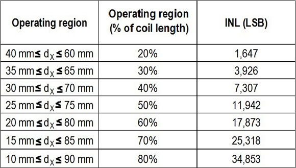
Table 3: Integral non-linearity at different operating regions.
The output code can be translated to travel distance by calculating the best-fit curve through the output response. System accuracy requirements dictate the minimum polynomial degree and, thus, the required processing power of the microcontroller. The output code can be translated to travel distance by employing a look-up table. This approach requires little processing power, but requires additional memory for the look-up table.
Summary
Inductive sensing is an ideal sensing method for linear position sensing due to its contactless nature and high reliability. Shaping the AC-magnetic field of the sensor coil by employing a stretched-coil design and a rectangular target allows system designers to minimize space requirements for the target while designing systems with resolution in the micrometer range.
About the Author
Ben Kasemsadeh is a systems applications engineer who specializes in audio and sensing solutions. He works in Texas Instruments' Silicon Valley Analog group on inductive and capacitive sensing solutions for consumer, industrial, and automotive applications. Ben graduated with a Master of Engineering degree in Electronics and Software Engineering from the University of Edinburgh, UK. For questions about this article, Ben can be reached at [email protected].
Related Stories
Where Does LVIT Technology Fit In The Sensor World
MDT Releases Ultra-high Sensitivity TMR Magnetic Switch Sensors at Sensors Expo
High Reliability Sensing Solution Based on Advanced Magnetostrictive Technology
See Gill's Inductive Position Sensor Technology at Sensors EXPO 2015