
 he word bandwidth is often used interchangeably with the term sample rate. However, since bandwidth applies to analog systems and sample rate applies only to digital systems, the two expressions are far from synonymous. This confusion of terminology can in fact lead to a misunderstanding of a given system's performance and may result in the purchase of a measurement system inadequate for the job at hand..
Analog System Bandwidth
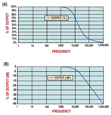 Figure 1. The transfer function of a single-pole, low-pass analog filter can be expressed as a percent of input (A) or as the amount of attenuation (B). A signal passed through an analog filter that has a bandwidth equal to the frequency of the applied signal is attenuated to 70% or 3 dB of its input value. |
The system designer's question is, "What bandwidth is required to meet my error budget?" The oft-quoted recommendation is that 10× your maximum signal frequency makes the measurement system bandwidth an insignificant contributor to error. The magnitude of this error is a function of the ratio of the measurement system bandwidth to signal frequency. For ease of understanding and analysis, a single-pole low-pass response is considered.
Defining:
| |
(1) |
the following formulas for a single-pole rolloff response apply:
| |
(2) |
| |
(3) |
It is desirable for r to be as large as possible. As r increases toward infinity, the error approaches 0. The error equation is plotted in Figure 2.
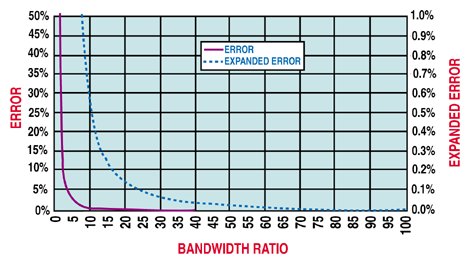 Figure 2. The error in a measurement system can be expressed as a function of the ratio of the measurement system bandwidth to the input signal frequency. The second vertical axis expands the error scale for higher values of bandwidth ratio. |
For higher values of bandwidth ratio (and lower errors), a second vertical axis is used to expand the graph. In this case, if you consider the standard recommendation of a bandwidth ratio of 10, the error is 0.5%. This may or may not be significant, depending on your system requirements.
Digital System Sample Rate
In a digital system, the input is sampled and the output is updated at a predefined rate. In between the samples, the input can change and the change will not be reflected in the measuring system output. If the input changes very quickly (or the sample rate is very slow), it is possible for changes in the input to be missed entirely. A digital system must sample at a fast enough rate to capture the changes on the input to an accuracy that matches the system performance requirements.
The bandwidth of the analog components is typically not a concern in a digital system; instead, the speed performance is most likely limited by one of the following:
The ratio of the sample rate to the maximum frequency of the changes in the input (a term I call the oversampling ratio)
The time latency from input to output; this is a fixed delay that occurs in updating the output and is usually expressed as a number of samples of delay
The effects of digital sampling can best be understood by considering examples of various input frequencies and sample rates. For measurement of periodic motion, if the sensor response is plotted on an oscilloscope it will often look similar to a distorted sine wave. Therefore, sine waves have been used to display the signal to be measured.
Example 1. Input Frequency at 960 Hz, Sampled at 5 kHz. The dots on the waveform in Figure 3 represent the data points that a digital system may have acquired.
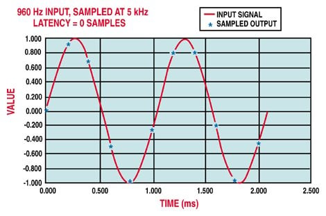 Figure 3. This is a possible result of a digital measurement system sampling a 960 Hz in-put signal at 5000 sps. The points representing the sampled output show how much of the input signal, particularly the peaks, may actually be missed if the input is not sampled often enough. |
Two effects should be noted from the graph:
At an oversampling ratio of 5.2, the output signal does not exactly follow the input. This effect is always present to some extent in a digital system, but can be minimized by a higher oversampling ratio.
The output does not appear cyclically consistent. Note that where the cycle minimums are closely captured for the two cycles shown, the maximum signal excursions appear to be missed. With multiple sine waves captured, eventually the maximum would be captured and the minimum missed. The reason is that the input wave is not sampled at a rate that is an integral multiple of the input frequency. Because the input frequency is rarely known and the sample rate cannot be adjusted, it is very likely that cycle-to-cycle sample points will not match up.
Example 2. Input Frequency at 1050 Hz, Sampled at 10 KHz. Observing Figure 4 and considering the same two effects as before:
At an oversampling ratio of 9.5, the output signal more closely follows the input, and the error in missing the maximum or minimum of the input signal has been reduced. This error can never be reduced to zero, but it is the goal of the system designer to determine the minimum sample rate that will reduce the error to a level that is small compared to the signal being measured.
The output does not appear cyclically consistent. Note that for one of the cycles the maximum appears to be missed, but for the next cycle it is captured near its peak excursion. This is similar to the previous example except that as a result of the sampling occurring at a higher rate, the discrepancy has also been minimized. Since the input frequency is rarely known and the sample rate cannot be adjusted, this is very likely a real-life scenario.
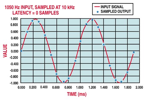 Figure 4. Similar to Figure 3, this is a possible result of a digital measurement system sampling at a 1050 Hz input signal at 10,000 sps. The higher oversampling ratio reduces the maximum error associated with capturing the peak of the waveform. |
Maximum Instantaneous Error in a Digital System
To determine the magnitude of the sampling error in a digital measuring system, you should choose the two sample points nearest the maximum or minimum so that they are equally spaced from the peak. The maximum potential error as a function of oversampling can then be determined analytically. Figure 5 shows the conditions for a maximum error using an oversampling ratio of 5, with the maximum error occurring at the two sample points near the peak of the waveform.
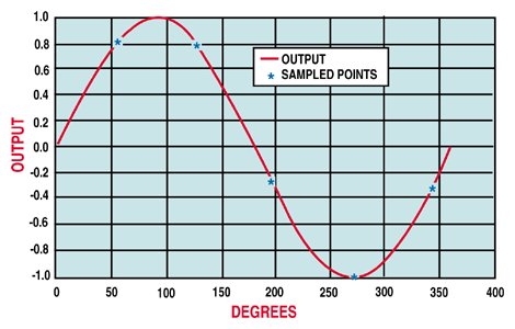 Figure 5. To determine the maximum error in digitizing the peak of a sine wave, assume that the two closest points are equally spaced from the peak. The error is the difference between the voltage at the sample point and the actual peak of the waveform. |
In this case, the sampled signal occurs at ~81% of the peak, resulting in an error of 19%.
As would be anticipated, for higher values of oversampling the error is reduced. Figure 6 plots the maximum error as a function of the oversampling ratio.
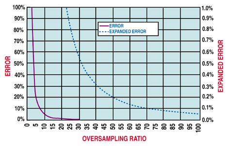 Figure 6. This graph demonstrates the way the maximum peak sampling error is reduced as the oversampling ratio is increased. An oversampling ratio of 10, the oft-quoted recommendation, could result in a 5% error in determining the peak of the waveform. |
For higher values of oversampling (and lower errors), a second vertical axis was used to expand the graph.
It is particularly interesting and important to note that standard practice often recommends an oversampling ratio of 10. In this case, the potential maximum error for a single-cycle sampling could be as high as 5%. Likewise for a potential maximum error of <0.5%, the oversampling ratio must be at least 32.
How Fast Do You Need to Sample?
1. Determine how much error can be tolerated when measuring the minimum and maximum displacements. Locate this point on the vertical axis in the maximum error vs. oversampling ratio graph. Follow this point to the horizontal axis to determine the minimum amount of oversampling required.
2. Determine the maximum frequency of the motion that needs to be characterized. Multiply this frequency by the oversampling ratio determined in Step 1. This is the minimum sampling rate that must be used to measure the input signal.
Performance Limitations Based on Latency from Input to Output
As mentioned earlier, the delay in updating the output must also be considered when evaluating a digital measurement system. The previous two examples of oversampling ratio will be considered with the added effect of time latency in the output.
Example 3. Input Frequency at 960 Hz, Sampled at 5 kHz, Time Latency of Two Samples. Note that the same errors of Example 1 are still present, but the output is shifted (delayed) due to the signal processing delays. Figure 7 more fully demonstrates the sampled nature of digital systems because the output points are not lying on top of the input sine wave. Remember that the data you observe are only from the sampled output points.
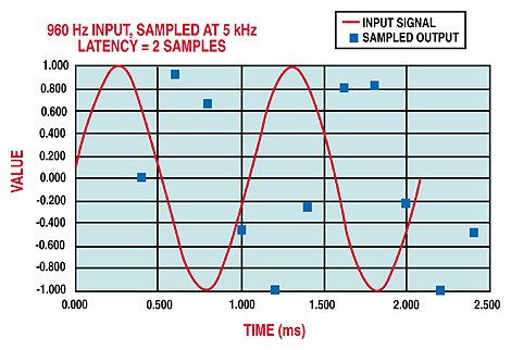 Figure 7. Another side effect in a digital measuring system is the latency from input to output. The configuration shown here is the same as in Figure 3, except that the output is delayed by two samples. With the sampled points not superimposed on the input signal, the discontinuous nature of digital sampling is readily apparent. Figure 7. Another side effect in a digital measuring system is the latency from input to output. The configuration shown here is the same as in Figure 3, except that the output is delayed by two samples. With the sampled points not superimposed on the input signal, the discontinuous nature of digital sampling is readily apparent. |
Example 4. Input Frequency at 1050 Hz, Sampled at 10 kHz, Time Latency of Two Samples. Note that the same errors of Example 2 are still present, but the output is shifted (delayed) due to the signal processing delays. The higher sample rate (compared to Example 3) has the effect of reducingboth the sampling and the time latency errors. The higher rate of oversampling allows you to more easily see the pattern of the input sine wave (see Figure 8).
Latency delay may or may not be a problem, depending on the application. If the measuring system is simply measuring the extremes of motion, the latency delay is not a problem. If, however, the measurement is a part of a control loop, the latency delay must be considered and could play a significant role in determining the stability of the control system.
Applications and Examples
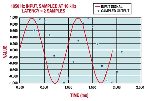 Figure 8. As the oversampling ratio is increased, the delay from input to output is decreased and the waveform reproduction is improved. Even at an oversampling ratio of ~10, there can still be significant error in capturing the peak of the waveform. |
 Figure 9. Measurement of runout in a rotating shaft is a good example of an application where peak measurement errors must be considered. The ideal case is a perfectly circular shaft rotating about its center (A). The measurement system will show a flat DC output. Figures B, C, and D highlight application problems that the measurement system will detect. |
Application 1. Runout in Rotating Shafts. A typical application of a position-measuring system is to measure the runout in a rotating shaft. This measurement would be useful for:
Determining system alignment and quality of assembly
Bearing wear
Dynamics of the rotating shaft, such as shaft growth, harmonics, bend-ing/material properties, and temperature effects
Figure 9A shows a perfect systema circular shaft rotating about its center. Figures 9B, C, and D show other types of error that may occur in a typical application. For Figure 9A, the gap from the sensor to the shaft is unchanging. The output of the measurement system will be a stable DC value. For Figures
9B, C, and D, the sensor-to-shaft gap is constantly changing. If the sensor response is plotted on an oscilloscope, it will look similar
 Figure 10. Measurement of reciprocating motion is another good example of an application where peak measurement errors must be considered. The large motion of the target may cause the sensor output to saturate when its position exceeds the sensor's measurement range. |
to a distorted sine wave. To measure shaft runout it is important that the measurement system be able to capture the peaks of the sine wave response. All of the previous concerns regarding the error as a function of oversampling ratio apply in this application.
Note that the frequency of the distorted sine wave output may be 2× the speed of the shaft rotation. This is more easily understood by looking at the ellipse and noting that a peak and valley occur two times for each shaft revolution. Unless the rotating shaft is keyed and it is desirable to know the relationship of the maximum or minimum runout location with respect to the key, time latency in the output is not a problem and can be ignored.
Application 2. Reciprocating Motion. From the standpoint of a digital system, this application is very similar to shaft runout. Figure 10 illustrates a typical reciprocating motion application: measurement of piston motion. This application is unique because the target does not necessarily remain in the sensor's dynamic operating range. When the target is outside the range of the sensor, the measuring system output may be saturated at the maximum value. The result is a sine wave type of motion, with the top of the waveform clipped at a fixed level. Figure 11 is included to give an idea of how the digitized results may look.
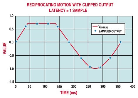 Figure 11. The waveform is plotted for reciprocating motion when sampled with a digital system at an oversampling ratio of 10. The negative peak sampling error is similar to the previous examples and should not be overlooked. |
An oversampling ratio of 10 is used for convenience. All of the previous concerns regarding the error as a function of oversampling ratio pertain tothis application as well. As before, time latency in the output is probably not an issue and can be ignored.
 Figure 12. Sometimes an application requires the measurement system to be sensitive to one effect and insensitive to others. In this case, the average gap between the rotating plates needs to be measured and the wobble that occurs during rotation needs to be ignored. A digital filter in a digital measurement system can often be tuned to accomplish this task. |
Application 3. Gap Between Rotating and Stationary Plates. In this application (see Figure 12), the gap between the rotating and stationary plates is to be controlled. It is assumed that the rotation rate is significantly faster than the rate at which the plate gap changes. If the plates are not parallel, the sensor will once again see a sine wave type of motion. The desired control is to keep the average plate spacing at a fixed value.
At first glance, this application looks similar to the previous examples. It highlights one of the strengths of a digital measurement system: digital filtering. Figure 13 shows the sensor signal and the system output for a plate rotation of 1000Hz. Two different digital filters are implemented to show their effects.
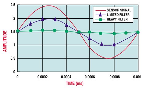 Figure 13. A digital filter can be used to remove the wobble between the two plates of Figure 12. In this application, there is no need for a high sampling rate, provided that rate is not synchronous with the input signal. Figure 13. A digital filter can be used to remove the wobble between the two plates of Figure 12. In this application, there is no need for a high sampling rate, provided that rate is not synchronous with the input signal. |
The measuring system should ignore the wobble and give a value of the average plate separation, which in this case is 1.5 units. A digital system with a programmable digital filter is a real advantage here. By programming the filter to a low frequency (heavy filter), the wobble in the plates can be filtered out. If the digital system has sufficient flexibility, the plate wobble can be attenuated to the point that it is hardly noticeable.
For the graph, an oversampling ratio of 10 is used for convenience; in the application, however, the oversampling ratio is not a significant factor provided the sampling and rotation rates are not synchronous or multiples of each other. The digital filter will cause the discrete points in the wobble to be averaged out. Thedigital sampling system need only be fast enough to track the actual up and down motion of the plates, not the speed of rotation.
Summary
In each of these applications, unless the system response is monitored on an oscilloscope it is important to recognize that the signal is usually digitized somewherein the measurement system itself, in an A/D acquisition card in a computer, or in a peak detection circuit in a DVM. Understanding the limitations in a digital measuring system will allow the user to specify a system adequate for the allowed error budget.
The examples and graphs given here provide the tools necessary to determine how fast you need to sample. Some points to consider:
Recognize that every measurement system has some type of error associated with it. Analyze the specific application to define the requirements and allowable errors.
Determine whether an analog or a digital system is appropriate for your application. Using the graphs, determine the bandwidth requirement for an analog system or the sample rate requirement for a digital system.
Be careful about confusing the specifications bandwidth and sample rate. The terms do not mean the same thing and cannot safely be used interchangeably.
Be cautious about applying rules of thumb or general solutions to your specific application. What is acceptable for another user may not beadequate for your needs.
Each applicationand the amount of error it can toleratemust be examined on its own merits. Digital systems, when compared to analog systems, provide many advantages but may also have some limitations depending on the actual application. You need to understand these performance tradeoffs when you make a decision on the type of measuring system. If in doubt, consult an application engineer to assist you in understanding how these tradeoffs apply to your own unique application.