Designing and Building an Eddy Current Position Sensor

The experience essential to successfully designing eddy current sunsors can be readily acquired because printed circuit sensors are easily and cheaply prototyped and only basic electronic instruments are needed for testing.

---

Steven D. Roach, Hewlett-Packard, Electronic Measurements Division

Photo 1. In the radial and thrust magnetic bearings shown here, three differential eddy current probes from Kaman Instrumentation Corp. (Colorado Springs, Colorado) monitor X,Y, and Z motion to a precision of <0.0001 in. The visible components are (from left) motor jack shaft; flexible coupling (black); left thrust housing and stator; thrust disc with shims for setup; right thrust housing, stator, and thrust probes; radial eddy current probe assembly; radial magnetic bearing housing and stator; auxiliary bushing assembly; and pump drive shaft. (Photo by George Gillies, courtesy of ROMAC).

Eddy current sensors are widely used for noncontact position, displacement, and proximity measurement. Operating on the principle of magnetic induction, these detectors can precisely measure the position of a metallic target, even through intervening nonmetallic materials such as plastics, opaque fluids, and dirt [1]. The sensors are inherently rugged and can operate over wide temperature ranges in contaminated environments that would defeat optical, acoustic, and even capacitive devices. One of the more exotic applications of eddy current sensors is that of supplying position feedback in magnetic bearings (see Photo 1 and sidebar). In a magnetic bearing assembly, a rotating shaft is suspended in a magnetic field to achieve wear-free and nearly frictionless rotation. For bearing stability, eddy current sensors are frequently used to provide position feedback to the magnet controller.

Practical eddy current sensors vary in diameter from a few millimeters to a meter and have maximum sensing ranges roughly equal to the radius of the coil. Linearity is typically 1% of the sensing range and noise levels of 1 ppm_rms/√Hz are common. Temperature drift ranges from ~100 ppm/°C to 1000 ppm/°C. A small sensor can resolve nanometer-size displacements and measure a 1 mm span to 10 microns total accuracy. Bandwidths of 50 kHz are readily achieved.

Figure 1. An AC current in the sensor coil generates an oscillating magnetic field, which induces eddy currents in the surface of the target. The coil impedance changes with standoff and is converted to a linear output by the sensor and signal processing electronics.

Physics and Behavior
An eddy current displacement sensor consists of four components (see Figure 1): the sensor coil, the target, the sensor drive electronics, and a signal processing block, which can be a circuit or a microprocessor algorithm.

When the sensor coil is driven by an AC current, it generates an oscillating magnetic field that induces eddy currents in any nearby metallic object, designated the target. The eddy currents circulate in a direction opposite

Figure 2. An eddy current sensor can be modeled as a transformer (A) with a coupling coefficient that depends on standoff. The model can be simplified to an inductor and resistor (B) that both depend on standoff, x.

that of the coil, reducing the magnetic flux in the coil and thereby its inductance. The eddy currents also dissipate energy, increasing the coil's resistance. As shown in Figure 2(A), the coil and the target constitute the primary and (shorted) secondary of a weakly coupled air-core transformer. Movement of the target changes the coupling, and this movement is reflected as an impedance change at the terminals of the coil.

The air-core transformer model is physically accurate, but for purposes of circuit design, a lossy inductor is simpler and more useful. In Figure 2(B), the complex impedance of the sensor coil is represented a series LR circuit. Both inductance, L, and resistance, R, change with target position, or standoff. As the target approaches the coil, the inductance goes down and the resistance usually goes up. The inductance changes by as much as

a factor of five, providing the physical basis for sensing the target position.

The inductance and resistance are important characteristics of the sensor because they correspond directly to physical mechanisms and can be used directly in circuit design and simulation. However, the quality factor, Q, is more directly connected to the ultimate performance of the sensor. Q is defined as:

(1)

where:

ω = operating frequency of the sensor in radians per second

Q depends on the standoff, x, because both L and R are functions of displacement. The higher the value of Q, the more purely reactive the sensor. High Q leads to high accuracy and stability. The specific value of L is of secondary

Figure 3. Measurements on a 38 mm dia. PC sensor at 1 MHz show how inductance, resistance, and Q are affected by target displacement. The inductance changes rapidly when the target is close but the response decays significantly at one coil radius.

importance since it is constrained only by the need for a manufacturable coil and a practical circuit design that burns a reasonable amount of energy at a reasonable frequency. The specific value of R is of even less interest because R is an undesirable parasitic effect in the first place.

Figure 3 shows how L, R, and Q depend on target standoff. The data come from real measurements on a 38 mm dia., air-core PC sensor with an aluminum target. The measurements were made on Hewlett-Packard's HP4285A LCR meter at 1 MHz. Note that the displacement has been normalized to the sensor radius (19 mm) so that the graph qualitatively depicts the behavior of sensors of all sizes. As standoff increases, the inductance increases by a factor of four, the resistance decreases slightly, and as a consequence the Q increases. The change in all three parameters is highly nonlinear and each curve tends to decay roughly exponentially as standoff increases. The rapid loss of sensitivity with distance strictly limits the range of an eddy current sensor to ~1/2 the coil diameter and constitutes the most important limitation of this type of sensing.

Figure 4. Target conductivity affects the response of the 38 mm PC sensor (A). A stainless steel target produces much higher eddy current losses and higher resistance when the standoff, x, is small. The inductance is much less sensitive to conductivity In (B), the Q values of aluminum and stainless steel are plotted against standoff, x.

The coil's impedance is also affected by:

• Target size, flatness, and thickness
• Target material properties, especially conductivity and magnetic permeability
• Temperature of the target and the coil
• Coil geometry and DC resistance
• Operating frequency

Figure 4 shows the effect of target material for an aluminum and a stainless steel target. The steel target has ¹/₂₈ the conductivity of aluminum, resulting in higher eddy current losses and higher resistance, especially at close spacing. The target conductivity scarcely affects the inductance. Neither resistance nor inductance depends strongly on the target at large sensing distances where the coil interacts only weakly with the target.

Figure 5 shows the sensor's response to frequency. First note the resonant behavior at 7 MHz, which is caused by the cable and interwinding capacitance. The frequency where the inductance peaks is called the self-resonant frequency (SRF), and the sensor must be operated below it to look like an

Figure 5. The frequency dependence of the 38 mm PC sensor shows that the Q increases with frequency until the coil becomes self-resonant. With this graph we can find an operating frequency that maximizes Q while staying well below self-resonance.

inductor at all. We want to operate the sensor at high frequency to maximize Q, but the frequency must remain at least a factor of three below the SRF. Since these are opposing requirements, the choice of operating frequency is clearly an opportunity for optimization. Practical frequency values for air core coils typically lie between 100 kHz and 10 MHz.

Temperature drift proves to be the critical source of error in eddy current sensors and arises from a complex set of factors. Both the inductance and resistance have positive temperature coefficients that are dependent on frequency. For the 38 mm PC coil operating at 1 MHz, for example, inductance increases at 88 ppm/°C. and resistance increases at 2400 ppm/°C. (Temperature drift will be examined in detail in a later article.)

Target Selection
The response of an eddy current sensor depends on both the conductivity and the magnetic permeability of the target. In some applications the designer is free to choose the target material; in others, the target is part of a machine or assembly over which the designer has no control. High-conductivity, nonmagnetic metals such as aluminum or copper make the best targets. Magnetic metals are also good choices, even though the sensor response is a mixture of eddy current and magnetic reluctance. Magnetic reluctance describes the way in which magnetic material modifies the effective permeability in a magnetic circuit. As a magnetic target approaches the coil, eddy currents reduce the inductance, while reluctance increases the inductance. Since these effects are in opposite directions, they may cancel each other. The net result is an easily avoidable null point in the sensor response at small standoff values.

The skin effect, or tendency for AC current to flow in the surface of a conductor, applies to both the coil and the target. Due to the skin effect, the current density in the target drops exponentially with distance from the surface. Skin effect is characterized by the skin depth, the distance at which the current density drops to 1/e of its surface value. The expression for skin depth in a conductor is given by:

(2)

where:

δ = skin depth (meters)
ω = radian frequency (radians/second)
μ = magnetic permeability (henries/meter)
σ = conductivity (siemans/meter)

For nonmagnetic materials, µ = µ_o = 1.26 x 10^-6 H/m. Table 1 shows skin depths in several materials for frequencies of interest in sensor design. Notice that the lower the conductivity and frequency, the more deeply the eddy currents penetrate the target. If the target is at least two skin depths thick, thickness is essentially eliminated as a factor in the measurement [2]. This rule-of-thumb, however, is extremely conservative.

TABLE 1

Skin Depth () in Microns for Various Metals and Frequencies
Metal	Conductivity (x 106 S/m)	Conductivity relative to Cu	Skin depth (µm)
			10 kHz	100 kHz	1 MHz	10 MHz
Copper	58	1.000	660	210	66	21
Aluminum	38	0.655	820	260	82	26
304 SS	1.3	0.022	4400	1400	440	140
Titanium Alloy	0.59	0.010	6600	2100	660	210

Several target characteristics other than thickness, conductivity, and permeability affect sensor behavior in ways that are difficult to predict analytically. Differences are seen if the lateral dimensions of the target are less than twice the sensor diameter, the target is curved, or its surface roughness is comparable to the skin depth. Though these situations are difficult to model, all can be accommodated with measurements by building a prototype sensor and measuring its response with an LCR meter. A versatile multifrequency instrument such as the HP4285A is extremely valuable for sensor design because it displays L, R, and Q directly with enough sensitivity to measure even minute effects such as temperature drift.

Sensor Design
The design of a nearly optimal eddy current sensor is surprisingly easy. We first need to establish some intuitive guidelines and a set of simplified design equations. Measurements of the prototype sensor with an LCR meter then provide highly accurate and detailed data for the design of the electronics.

If small size is the primary goal, sensors based on wirewound coils are the best choice. The fine magnet wire used in wirewound coils increases the sensor Q by maximizing the number of turns while minimizing the resistance. The magnet wire must be packed in perfect layers (usually by hand) under a microscope. The coils are then inserted in a machined protective holder and potted with epoxy to mechanically stabilize the windings. A wirewound sensor is a labor intensive product, and typically costs more than $100.

When cost is the primary consideration, coils printed on a PCB deliver excellent performance for a fraction of the cost of a wire wound sensor. The advantages of printing the sensor coil include:

• Prototyping. Tooling costs are only a few hundred dollars. A single prototype run can produce a large number of variations on the sensor design.
• Manufacturing. PCB processes are highly automated, standardized, and widely available. PC board processing scales well from tens to millions of sensors.
• Cost. Coils cost less than $1.00 in volume, but the cabling and connectors can easily dominate the overall price.
• Performance. The performance competes with wirewound sensors for larger diameters (>10 mm).
• Special configurations. Arrays of sensors and sensors on flex circuit material create unique application opportunities.

The primary tradeoff with printed sensors is size. It is difficult to print a coil <10 mm dia. on a PCB and still match the performance of a wirewound sensor. Table 2 outlines the most important factors and tradeoffs in the design of an eddy current sensor.

TABLE 2

Factors in Sensor Design [2]
Factor	Why	How	Tradeoffs
High-quality factor, or Q	Fundamental determinant of temperature stability, power consumption, noise; do anything possible to increase Q	Increase frequency and inductance, decrease resistance; use a wire-wound coil for small sensors	Difficult to achieve high Q with small sensors
High inductance	Increases Q and reduces power	Use more turns in the coil, a larger diameter sensor, or a ferrite core	High inductance is often accompanied by low self-resonant frequency
Low resistance	Increases Q and reduces power	Use more conductive coil windings, larger wire or thicker traces, keep temperatures low	Frequency trades off with the need for high inductance
Optimal coil size	Maximizes sensitivity to displacement	For highest accuracy and stability choose radius=3 x range; a small sensor has small range, too large a sensor has reduced sensitivity	The larger the sensor the larger the "spot size" or area of the target measured by the sensor; the larger the sensor, the larger the required target dimensions
Flat, disc-shaped coil configuration	Maximizes sensitivity by placing all of the turns close to the target	Use a printed coil	Flat coil limits the number of turns, reducing inductance
Operate at high frequency	Increases Q and redeuces power in the sensor; increases sensing bandwidth	Reduce interwinding and cable capacitance	Must stay below the self-resonant frequency; high frequency usually increases power in the electronics
Minimize cable length	Reduces cable noise, temperature drift, and cost of cabling; increases the self-resonant frequency; allows use of lower quality, cheaper cabling	Place the critical circuits in a pod close to the sensor or load electronics on back of printed coil	Placing electronics on or near the sensor limits the temperature range

A complete sensor typically has a cable joining the coil and the electronics. The cable can be coaxial, twisted pair, ribbon, or traces on a PCB. The cable affects system design and performance in several ways because all cables have inductance, capacitance, and DC resistance. The inductance of the cable adds to that of the sensor. Because the cable inductance is static (not sensitive to displacement), it reduces the sensor's net sensitivity. The cable capacitance forms part of the resonant circuit network, so any instability in the cable capacitance degrades measurement accuracy. Changes in cable capacitance with temperature and cable movement produce measurement errors. A common problem with eddy current sensors is noise traceable to cable vibration. Eddy current sensors can be so sensitive that a hand moving near a twisted-pair shows up as an observable displacement error, so the highest performance sensors require fully shielded coaxial cable. The resistance of the cable is in series with the sensor coil and contributes to a reduction in Q and to temperature drift. For the best performance, we must use high-quality microwave coaxial cable such as RG-178 or RG-316. These cables have a highly stable Teflon dielectric and low capacitance.

When price is an important consideration, and some stability can be sacrificed, twisted-pair or ribbon cabling is adequate and can be used with very inexpensive connectors. Twisted-pair can be soldered to a printed coil sensor directly, eliminating at least one set of connectors. Measurement errors due to cabling can be greatly reduced by placing the sensor interface circuitry on the back of a printed circuit coil. Even though the circuit operates in the coil's magnetic field and the coil "sees" the circuitry, performance is not seriously affected. It is important, though, to avoid a ground plane or any large loop areas in the circuit because the sensor would see these as a second target. With the sensor circuitry integrated with the coil, we still must deliver power and retrieve the output signal through cabling, but this cable in no way affects the accuracy of the measurement.

To establish guidelines for the design of the sensor we need a preview of the sensor drive circuitry. The circuits developed in the "Circuit Design" section of this article place the sensor in an oscillator loop where it is resonated with a capacitor. The frequency of oscillation (resonant frequency) is dependent on target displacement and is the output of the circuit. In an LC oscillator the frequency is proportional to 1/√LC. The design of an air core sensor with a printed circuit coil follows these steps:

  1. Set the outer coil radius, r_o. We need:
r_o > 2 x sensing range for a typical design
r_o = sensing range for an aggressive design

  2. Choose a manufacturing technology for the coil. The manufacturing technology determines the width, w, thickness, t, and pitch, p, of the traces that make up the coil windings.

  3. Calculate the number of turns that can be packed on a single layer.
The outer coil radius, r_o, was determined in an earlier step.
The inner coil radius, r_i, should be at least ¹/₃ the outer radius.

The number of turns per layer is:

(3)

  4. Calculate the unloaded inductance using Burkett's inductance equation [3]. The unloaded inductance is the inductance of the free coil with no target. Assume one layer for now.

(4)

  5. Calculate the cable capacitance, C_CABLE, from the cable length and the manufacturer's specification of capacitance per unit length. Assume that the interwinding capacitance, C_IWC, is zero for a single layer coil. For a two-layer coil, estimate C_IWC to be ¼ the parallel plate capacitance, calculated as if the windings were solid sheets of metal. Thus, for a two-layer coil:

(5)

where:

ε_r = relative dielectric constant (a dimensionless number; ε_r = 4.2 for FR-4 PC board)
ε_o = permittivity of free space = 8.86 × 10^-12 F/m
h = thickness of coil (meters)

  6. Estimate the self-resonant frequency:

(6)

  7. Choose the operating frequency. For the LC oscillator circuit, the minimum frequency coincides with the maximum inductance and occurs at maximum standoff. The maximum inductance is given approximately by Equation 4. We want the maximum frequency, which is typically about twice the minimum, to be no more than ¹/₃ the SRF so that the cable and interwinding-capacitance have only a small effect. With these considerations we have:

(7)

(8)

(9)

where:

C = total parallel resonant capacitance and L comes from Equation 4. Equation 9 can be used to calculate the capacitance required to resonate the sensor at the desired frequency.

  8. Calculate the DC resistance of the coil:

(10)

where:

l = length of the coil windings
ρ = 1/σ = resistivity of the coil windings
w = width of traces of coil windings
t = thickness of traces in coil windings

  9. Estimate the worst-case AC resistance, which is higher than the DC resistance because of the skin effect and proximity effect.

RAC = 2RDC

(11)

  10. Calculate the unloaded Q. (The Q of the free coil with no target.)

(12)

We need:
Unloaded Q > 15 for a typical design
Unloaded Q > 5 for a design with a Q >15

If Q is not high enough, consider adding additional layers to the coil. Doubling the number of layers doubles the number of turns, which quadruples the inductance while only doubling the resistance. The Q therefore roughly doubles. Also, follow the guidelines in Table 2 to increase Q.

  11. Is the unloaded inductance acceptable? If the inductance is too high (a rare situation except for large coils), the resonant capacitance may be too low, allowing cable and interwinding capacitance to dominate the sensor behavior. If the inductance is too low (a common problem, especially for small coils), the circuits may burn excessive power or require an impractically high operating frequency for acceptable Q.

We need:
1 µH < L < 100 µH for a typical design (but aim for L > 10 µH)
L < 1 µH for an aggressive design

If the inductance is too low, increase the number of turns by using a finer pitch PC technology, adding layers, or using hybrid integrated circuit technology.

  12. Build a prototype of the coil and measure it on an LCR meter to confirm the design and to collect data on L(x) and R(x) (x = standoff). The data will be used to design the electronics. To make these measurements, attach the target and sensor to a micrometer with an appropriate fixture.

Circuit Design

Figure 6. Adding a capacitor to the sensor creates a resonant sensor network that magnifies the sensitivity of the impedance to target displacement. (jω) = V(jω) / I(jω) = the complex impedance of the circuit.

The challenge in circuit design for eddy current sensors is to develop an output that is linearly proportional to standoff and independent of temperature. The sensor converts displacement to a change in impedance, and the circuit converts the change in impedance to another electrical parameter such as the amplitude, phase, or frequency of an RF carrier. This signal must be demodulated, temperature-compensated, linearized, offset, and scaled. These steps may be carried out by a circuit, an algorithm, or a combination of both.

The basis for nearly all eddy current sensor circuits is shown in Figure 6, where the sensor coil is resonated with a capacitor. Resonance causes abrupt changes in the circuit impedance Z(jω), as shown in Figure 7, in which the middle point is x = 4 mm. In Figure 7(A), the magnitude peaks at the resonant frequency and the height of the peak depends on the Q, which in turn depends on the target displacement. In Figure 7(B), the phase shifts from +90 at low frequency to ­90 at high frequency.

Figure 7. The impedance, Z, of the resonant sensor network in Figure 6 depends on frequency and target displacement. Target standoff, x, changes the frequency at which the magnitude peaks (A) and the phase crosses zero (B), providing bases for position sensing.

The frequency of the phase transition depends on the inductance, which depends on the target position.

A common way to convert the displacement to voltage is simply to drive the resonant circuit with a current source at a fixed frequency and demodulate either the amplitude or the phase of the voltage that appears across the sensor. Both amplitude and phase detection are complex, requiring an independent oscillator, phase detector, low-pass filter, and analog postconditioning circuits.

With the goal of designing a position sensor of the lowest possible cost, consider the self-oscillating circuit of Figure 8. It is a straightforward gate oscillator using low-voltage CMOS logic gates. The two inverters produce

Figure 8. An LC gate-oscillator circuit with an eddy current sensor generates a frequency output that depends on the target standoff. A microcontroller can directly digitize the frequency by counting the output pulses.

a large, positive voltage gain, so the circuit oscillates at a frequency where the phase shift of the resonant sensor network is zero. The output is a square wave whose frequency is a function of displacement and which changes ~2:1 over the full practical range of standoff. Assuming that a microcontroller is already part of the host system, the advantages of the circuit in Figure 8 include:

• The output can be connected directly to the counter-timer port of the microcontroller and digitized simply by counting pulses. The microcontroller digitally linearizes, offsets, and scales the output using constants stored during calibration.
• Because every sensor component (the coil and all electronics) is under calibration, no costly, high precision devices are needed.
• The circuit operates on a single supply voltage at a few hundred microamps of current.
• The circuit requires 7 electronic components at a material cost of about $0.35. A PCB coil is on the order of $0.50 in volume. With the addition of the load and test costs, the cable and assembly labor, the entire sensor subsystem adds as little as $2.00 to the cost of a high-volume, microcontroller-based product.

The circuit in Figure 8 oscillates at the resonant frequency given by:

(13)

To find the component values for Figure 8 we first determine the desired operating frequency from the procedure described earlier. Then we solve Equation 13 for C_p and choose the nearest standard value. R_s determines the amplitude of the signal at the input of the first inverter as well as the power consumption. To minimize noise it is desirable to have the largest signal possible at the inverter input. The smaller the value of R_s, the larger the signal, but the greater the power consumption. At resonance, the impedance of the of the LC tank is purely resistive and is equal to:

(14)

R_s and R_res form a voltage divider, so the amplitude is given by:

(15)

where:

4/π • V_DD is the amplitude of the fundamental of the square-wave output signal. We need only consider the fundamental component because R_s and the LC tank form a bandpass filter centered on the frequency of oscillation. This filter attenuates all but the fundamental component to a negligible level. A good rule of thumb is that the peak-to-peak amplitude in Equation 15 should be at least half the supply voltage, V_DD, when the coil is unloaded (i.e., when the target is not present). With this guideline we would set R_s ≈ R_res, with R_res found for the unloaded case.

The higher the resistance at resonance (Equation 14), the less power it takes to drive the sensor. Notice that the resistance goes up and the power goes down for higher frequencies, higher inductances, and higher values of Q.

CMOS gate oscillators such as that in Figure 8 exhibit curious power dissipation characteristics. The first inverter operates part of the time with its input at the logic threshold. This places it in the so-called linear region, where it acts like a class B linear amplifier and conducts current directly from the power supply to ground. The higher the supply voltage, the higher the class B current, so the power in the circuit of Figure 8 increases rapidly with supply voltage. For example, going from V_DD = 2.0 V to 2.5 V increases the current by a factor of four. By placing a resistor between V_DD and the inverter power pin the circuit can be operated on higher supply voltages while maintaining low power consumption. The resistor drops the voltage on the inverters and provides negative feedback to limit the class B current. Of course, the decoupling capacitor should still be attached to the power supply pin of the chip.

A Model Sensor System Design

Figure 9. This 38 mm diameter PC sensor was designed and prototyped in ~2 hr. with the aid of a PC milling machine. Built on 0.76 mm (0.030 in.) circuit board, the traces are 0.5 mm wide with a 0.76 mm pitch, yielding a total of 34 turns on two layers.

The sensor shown in Figure 9 was fabricated to illustrate the complete design of a low-cost sensor system. It is an octagonal spiral milled on a numerically controlled milling machine designed specially for rapid prototyping of printed circuits. With this machine, a sensor coil can be designed and fabricated in <1 hr. The LCR measurements for this sensor with an aluminum target are shown in Figure 3. The circuit used is shown in Figure 8 with R_s = 10 kΩ , C_p = 910 pF, and V_DD = 2.0 V. R_s is a 1%, 100 ppm/°C metal film resistor, though a 5%, 200 ppm/°C resistor would have negligible effect on overall performance. C_p is a 5% NPO capacitor with ±30 ppm/°C temperature coefficient. The initial accuracy of C_p affects only the initial frequency and is normally calibrated out. The drift of C_p is very important, however, so an NPO capacitor or similarly stable capacitor must be used.

Figure 10. The frequency output of the gate oscillator changes by almost 2:1, or 1 MHz, over the 19 mm sensing range. This example uses the 38 mm PC sensor and an aluminum target.

Figure 10 shows the frequency output for the model sensor system. The data were taken with the aid of an HP53132A frequency counter. Since the total inductance shift in Figure 3 is 4:1, the frequency shift is the square root of that or 2:1. Operating between 1 MHz and 2 MHz, there is an impressive total frequency shift of almost 1 MHz.

The frequency is a highly nonlinear function of displacement, so linearization is essential. The empirically derived function:

(16)

Figure 11. For a range of 19 mm, the gate oscillator produces excellent linearity of 1% after correction.

with f_o = 981 kHz produces the linearized output of Figure 11. The linearity error is <1% of the 20 mm F.S. range, or 200 µm. Even better linearity could be attained by calibrating at a large number of points and using piecewise correction. The advantage of linearizing with Equation 16 over piecewise linear correction is that the constants, m, b, and f_o, can be obtained with only three calibration points: the end points and a point near the middle of the range. It is not even necessary to know the midrange point exactly since the calibration procedure need only place this point on a straight line between the end points.

Figure 12. At 280 mA and 2 V the gate oscillator burns less than 600 µW, qualifying as a micropower sensor. Eddy currents degrade the sensor Q, increasing the power and decreasing the amplitude when the target is close to the sensor.

Figure 12 shows the sensor amplitude and power supply current. Notice that the amplitude decreases for small values of standoff because the Q is dropping rapidly. The reduced Q also requires more drive current from the power supply. With a supply voltage of 2.0 V the worst case power dissipation is <600 µW. The power is so low that the capacitance of a 15 pF scope probe on the output increases the power by 20% due to charge pumping.

The frequency output of the sensor is highly nonlinear, changing some 125:1 in slope over the full. If the circuit noise and quantization error are roughly constant in terms of frequency, then they will not be constant in terms of displacement. In terms of displacement, both the noise and resolution vary in inverse proportion to the slope of the frequency curve, so they will vary by 125:1 also. If we measure frequency by counting N pulses over a gate time of T_g, the estimated frequency is fest = N/T_g. The quantization error is ±1 count, so the frequency resolution is Δf = 1/T_g. Clearly, the longer the gate time (and the slower the sample rate), the higher the resolution. Arbitrarily high resolutions can be reached by counting for longer periods. Noise is reduced at the same time because the counting process acts as a digital low-pass filter.

The resolution in terms of displacement depends on the slope of the frequency curve:

(17)

Figure 13. Displacement noise and quantization error increase as the target moves away from the sensor because the inductance change decays with distance. The noise and quantization are relative to a full-scale standoff of one coil radius and the frequency counter gate time is 100 ms.

Noise follows the same form as Equation 17, increasing for larger values of standoff. Figure 13 shows the resolution and noise of the model sensor for a gate time of 100 ms, or a digitizing rate of 10 sps.. The noise is ~20 Hz p-p as measured with the HP53132A counter with a 100 ms gate time. Most of the noise is at very low frequency (<1 Hz) and can be caused by vibration or temperature changes due to air currents. Notice that higher resolution and lower noise can be attained by simply limiting the maximum standoff.

A very good way to observe the noise is to display the output square wave on a digital oscilloscope and delay the scope by 1 ms. With the sensor operating at 1 MHz (a 1 µs period), the scope displays the phase noise accumulated over 1000 cycles. With the digital scope set to infinite persistence, the

Figure 14. The temperature stability of the gate oscillator compares favorably with some of the best commercial sensors. The temperature coefficient is taken relative to one coil radius.

trace will "paint" a band several nanoseconds wide. The width of this band divided by the delay time of 1 ms gives the relative noise. For example, 20 ns_p-p/1 ms is 20 ppm or 20 Hz at 1 MHz.

Figure 14 shows the temperature stability of the sensor and the electronics. The stability is poorer at large displacements because at large values of standoff the temperature stability suffers the same disadvantage as the resolution and noise. Limiting the sensing range can greatly improve temperature stability. Table 3 summarizes the measured performance of the model sensor for two values of full-scale range.

TABLE 3

Summary of Performance of the Model Sensor System
Performance Parameter	10 mm Range	20 mm Range	Units
Frequency range   Max.   Min.	1.88 1.05	1.88 1.00	MHz MHz
Linearity	1%	1%	of range
Quantization error   1 sps   10 sps   100 sps	17 14 11	15 12  9	bits
Noise, peak-to-peak   1 sps   10 sps   100 sps	14 13 12	12 11 10	bits
Temperature drift   Electronics   Sensor	-150 +300	-540 +1200	ppm of range/°C
Power supply   VDD   IDD   Power   Power supply rejection	2.0 280 560      7	2.0 280 560   18	V µA µW %/V

Conclusion
Eddy current sensors are advantageous for precision, noncontact displacement sensing where the range is relatively small. They are especially useful where the environment is dirty or sensing through intervening materials is required. In applications where a microcontroller is available, a high-performance eddy current sensor can be added to the system for a few dollars, using printed circuit sensors and manufacturing methods common to all electronic products.

Experience is essential to the successful design of eddy current sensors, but it is quickly gained because printed circuit sensors are easily and cheaply prototyped and only basic electronic instruments are needed for testing. The essential design calculations can be done with a desktop computer and a spreadsheet program. Future articles will investigate advanced computer-aided design methods for optimizing the sensor and advanced circuit designs for improved temperature stability.

References
  1. Scott D. Welsby and Tim Hitz. Nov. 1997. "True Position Measurement with Eddy CUrrent Technology," Sensors, Vol. 14, No. 11:30-40.

  2. J.H. Smith and C.V. Dodd. 1-5 Oct 1973. "Optimization of eddy-current measurements of coil-to-conductor spacing," Proc Annual Fall Conference of the American Society for Nondestructive Testing, Chicago, IL:1-15.

  3. Frank S. Burkett, Jr. 12-12 May 1971. "Improved designs for thin film inductors," Proc 21st Electronic Components Conference, Washington, DC:184-194.

SIDEBAR:

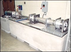
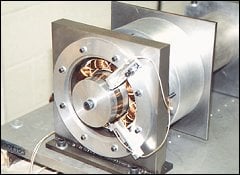
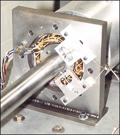
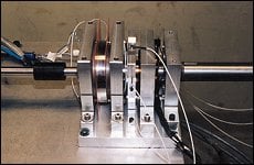
The ROMAC Research Facility Lloyd Barrett, the University of Virginia In a fault tolerance test platform, a 2-m-long mockup pump shaft is supported in three radial magnetic bearings and one magnetic thrust bearing. This apparatus is used to study fault tolerance strategies and has successfully demonstrated its ability to tolerate multiple simultaneous power amplifier failures as well as controller CPU failures. Seven single-sided eddy current probes made by Bently Nevada (Minden, Nevada) are used to measure shaft motion at the bearings for feedback to the controller. The controller bandwidth is ~1 kHz. (Photo by George Gillies, courtesy of ROMAC.) The Rotating Machinery and Controls (ROMAC) Industrial Program supports cooperative research efforts conducted by faculty, staff, and students in the Mechanical, Aerospace, and Nuclear Engineering and the Electrical Engineering departments at the University of Virginia. The ROMAC program emphasizes theoretical and experimental research in general areas of rotor dynamics, turbomachinery, structural dynamics, magnetic bearings, the application of automatic controls to the dynamics of rotating machinery, internal incompressible flows, the coupling of internal flows to the dynamics of rotating machinery, fluid film bearings, and seals. The interaction between industry and university The left and right end radial magnetic bearings on a fault test facility are shown in a close-up view. Two single-sided eddy current probes monitor X and Y motion to a precision of <0.0001 in. at a bandwidth of ~2 kHz. (Photos by George Gillies, courtesy of ROMAC.) professionals through the medium of ROMAC provides the university researchers with an understanding of practical industrial problems with rotating machinery while the industrial participants obtain very timely research results. The magnetic bearing research program, housed in the ROMAC laboratories, is one of the largest in the world. Experimental platforms include 12 magnetic bearing rigs ranging from a tiny artificial heart pump up to a 200 HP centrifugal compressor. The program's research covers the full spectrum of the technology, from hardware issues (system dynamics, magnetics, amplifiers, sensing, and controllers) to the the development of control methods. Lloyd E. Barrett is Professor and Laboratory Director, ROMAC Laboratories, Dept. of Mechanical, Aerospace, and Nuclear Engineering, the University of Virginia, Thornton Hall, McCormic Rd., Charlottsville, VA 22903-2442; 804-924-3292, fax 804-982-2037.