Angular Position Sensing with 2-Axis Hall ICs

By Lou Law Mar 1, 2003 1:00am

Whe 2-axis Hall sensor integrates a standard CMOS process and planar magnetic concentrators. Four sets of Hall elements are placed on the silicon die at the edge of a very small ferromagnetic disk concentrator consisting of a high-permeability and low-coercive-field ferromagnetic layer bonded to the surface of the chip surface. The flux concentrator converts the field components parallel to the device surface into a component perpendicular to it, allowing the use of conventional CMOS Hall technology in its fabrication. The perpendicular component of the magnetic field is strongest near the edge of the disk, where the Hall elements are located. Flux concentrators provide field magnification without amplifying the device noise.

Hall elements are located at the four quadrants of the disk to provide X and Y outputs (see Figure 1).

Figure 1. The integrated ferromagentic concentrator is located at the center of the silicon die and the Hall elements are at the edges of the disk (A). Parallel flux fields are converted to perpendicular flux fields that are sensed by the Hall elements (B). A layout detail showing the four sets of Hall elements with p/2 shift is shown in (C).

Only one Hall element is required for each axis, but additional gain can be realized and offset reduced by measuring the differential voltages from two devices at each quadrant position. The differential outputs from the X1, X2 and Y1, Y2 Hall elements are processed by the integrated electronic circuitry and include biasing, amplification, offset cancellation, and temperature stabilization functions.

Full-scale linear outputs of 2.5 V ±2.0 V can be obtained at field strengths as low as 20 mT (200 G). The V_x and V_y outputs are balanced with minimal offsets; because of the single-die construction they are not only matched, but also have excellent tracking performance. Several unique performance characteristics inherent in the technology make it especially well suited for precision sensing applications: a nonlinearity <0.1% and hysteresis <0.03%.

Figure 2. The 2-axis IC produces outputs proportional to the B_x and B_y field components of the magtnet rotating above the sensor.

Because they have only one sensing axis, conventional noncontact angular position sensors based on single-element linear Hall ICs are limited to a theoretical maximum of 180°. The 2-axis linear Hall IC can detect 360° of rotation and provide absolute position information over this range. As shown in Figure 2, a magnet, magnetized across its diameter, is attached to a shaft and rotated above the IC around the axis of the magnet and IC centerline. As the shaft is rotated, the IC senses the magnetic vector of the field from the magnet and generates signals V_x and V_y that are proportional to the sine and cosine signals, respectively. As shown in the following equations, a voltage representing the absolute angle,

, can be derived from calculating the arctan of V_x and V_y using a small 8-bit microcontroller or equivalent processor (see Figure 3).

Figure 3. The outputs from the 2-axis IC are processed by a microcontroller to create an output proportional to the angle of rotation (A). Linear output voltage is a function of V_x (cosine) and V_y (sine) (B).

V_x = S_x × B × cos

V_x = S_x × B × sin

(1)

The IC gain sensitivities, S_x and S_y, are closely matched and track over temperature. We can therefore assume that S_x and S_y are equal:

if S_x = S_y = S,
then V_y/V_x = S × B × sin

/S × B × cos

= sin

/cos

= tan

(2)

and therefore,

= arctan (V_y/V_x) = V_out

(3)

The arc tangent function repeats every 180° and becomes infinite at 90° and 180° when V_x = 0. This can be accounted for, however, by using the following equations:

(V_x >0, V_y >0),

= arctan (V_y/V_x)

(4)

(V_x = 0, V_y>0),

= 90°

(5)

(V_x <0),

= 180° + arctan (V_y/V_x)

(6)

(V_x = 0, Vy <0),

= 270°

(7)

(V_x >0, V_y<0),

= 360° + arctan (V_y/V_x)

(8)

The potential variability resulting from changes in S or B are canceled out by dividing V_y by V_x. Therefore, the

Figure 4. This is a cutaway view of a typical angular position sensor based on the 2-axis Hall IC.

analog output voltage representing the angle is independent of magnet strength, temperature effects, and gain sensitivity of the IC. The output becomes a function of the magnetic field vector orientation înly, and will always represent the absolute mechanical position of the magnet over the full 360° range. Figure 4 shows a typical 360° angular errror. Power can be removed and reapplied without losing the absolute position of the magnet.

The magnet creates a DC field that will project through any nonferromagnetic material, such as aluminum, 300 series stainless steel, and plastics. Because of this, the 2-axis IC and associated electronics can be mounted in a hermetically sealed metal housing that

Figure 5. The 2-axis IC and associated electronic circuitry located inside a nonmagnetic metal housing can also detect the rotation of a mechanism through a metal, such as the valve shown here.

mechanically isolates it from the rotating mechanism. Another advantage of this configuration is that it imposes zero ?drag? on the rotating mechanism. A sensor using this technology could, for example, measure the position of a valve inside a sealed housing if a magnet were to be mounted on the internal shaft and the sensor placed on the outside (see Figure 5).

Having to incorporate a microcontroller to calculate the angle might be considered a negative, but with the microcontroller and the 360° information from the IC, the potential sensor solutions are numerous and functionality is greatly expanded. Any custom output curve can be programmed; outputs can be analog, PWM, PPM, or serial data. Mechanical alignment of the magnet to the sensor can be eliminated by simply resetting the starting point within the 360° range.

Figure 6. The 2-axis IC can be mounted on the axis of rotation of a single-axis joystick to directly measure the angle of rotation. Two independent sensing circuits can be used to provide redundant outputs (A) and (B).

Single-Axis Joystick. The 2-axis linear Hall sensor offers a simple solution for noncontact single-axis joysticks. Figure 6 illustrates a configuration in which the magnet is mounted in the shaft of the stick handle and the IC is mounted on a PCB attached to the frame of the device. By placing a sensor on either side of the handle, a dual-redundant joy stick can be constructed. The IC is located on the centerline of the magnet axis. The angle of rotation can be acquired by calculating the arctan of V_x and V_y similar to the 360° rotary application described earlier. With the microcontroller and the 360° of position information from the sensor, numerous output curves can be generated and the need for mechanical alignment of the sensing device to the rotating handle be can eliminated:

V_out = arctan (V_y/V_x)

(9)

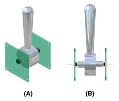
Figure 7. For joystick applications, the 2-axis IC can be gimbal mounted at the spherical center of rotation. The X and Y outputs are linear within ±30º (A). In another configuration, the IC is mounted on a ball joint, again with the IC at the spherical center of rotation (B).

2-Axis Joystick. Most 2-axis joy sticks measure their position by mounting two potentiometers to the shafts of a gimbal system and extracting the X and Y coordinates from the sensors. With one 2-axis IC mounted at the center of spherical rotation and a magnet mounted in the handle, simple, 2-axis, noncontact joysticks can be constructed (see Figure 7).

The X and Y outputs from the IC are proportional to the vector of the magnetic field. The profile of this vector is a sine wave with the field vector in the X,Y plane, being zero when the joystick is in its neutral position (see Figure 8).

Figure 8. The magnet is rotated around the two-axis IC located at the center of spherical rotation (A). The voltage output generated by the rotating magnet is a sine wave with zero output located at the joystick's center position (B). An expanded view of the sine wave shows the ~60º linear range centered around the 0º angle. The nonlinearity, shown in red, is <1% of F.S. (C).

A sine wave has a linear range of <1% nonlinearity over a 0°?60° range around the 0° angle. Because most joystick applications have a typical operating range of ±30°, the linear output voltage generated by this Hall sensor works well in simple, noncontact 2-axis joystick applications. No calculations are required, and the X and Y outputs are directly proportional to the magnet strength and IC sensitivity so can be used directly as shown in Figure 9. Depending on accuracy requirements, the output levels may have to be calibrated to the mechanical position to compensate for variability in B and circuit sensitivity.

Figure 9. Linear outputs from the 2-axis IC provide X and Y outputs from the joystick's ±30º stroke. The 2.5 V ±2.0 V outputs are referenced to the IC's 1/2 V_dd (2.5 V) reference voltage. The oututs are ratiometric to the supply voltage.

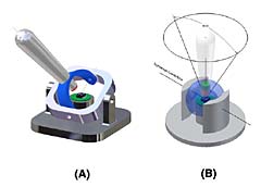
High-Resolution Sensor. Figure 10 illustrates a way to obtain higher resolution and improved accuracy in a rotary position sensor by using two X,Y ICs and two magnets.

Figure 10. A multipole and a single pole pair magnet are used to generate fine and coarse measurements of the angular position. The multipole sensor is located at the circumference of the magnet, and the coarse sensor is on the axis of rotation (A). The basic circuit to process the signals from the two ICs is shown in (B).

The magnet associated with the IC on the lower PCB is a single pole pair magnet that provides a coarse measurement by producing one electrical cycle of sine and cosine signals per revolution. The magnet associated with the IC on the upper PCB is a multiple ring magnet and provides a fine measurement by producing n electrical cycles of sine and cosine signals per revolution, where n = number of pole pairs (see Figure 11).

Figure 11. As can be seen in this graph, for every full resolution one cycle of sine and cosine signals is generated from the coarse sensor while eight cycles of sine and cosine are generated from the fine sensor.

Each electrical cycle has a resolution of 0.1°, so the total resolution for one complete revolution is 0.1°/n. If n = 8 pole pairs, the resolution becomes 0.1°/8 = 0.0125°, or 45 arc-seconds. The coarse information from the lower PCB is used to locate which sector (pole pair) of the multipole ring magnet is in front of the upper PCB IC.

Within one pole pair, or measurement range of 360°/n, the accuracy is also improved by n: accuracy = 0.5°/n and overall accuracy of one 360° revolution can be significantly enhanced with electronic calibration. The fine and coarse signals are processed by a microcontroller to generate an output with greater resolution and accuracy.

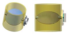
Compass. Another unique application is an electronic compass (see Figure 12), in which the IC is mounted over a mechanism that allows a free-floating magnet.

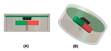Figure 12. A side view shows the north-seeking magnet just below the 2-axis sensor, which senses magnetic fields parallel to the magnet. As the magnet rotates, the sensor generates sine and cosine signals at the V_x and V_y outputs, which can be converted to the absolute position of the magnet (A). The Earth's field-seeking magnet is mounted on a low drag bearing assembly to allow free movement (B).

As the magnet rotates and aligns with the Earth?s magnetic field, it creates a field vector that is aligned with the orientation of the magnet. The magnet?s field strength is much stronger than Earth?s, which is only about 60 µT (600 mG) and too low compared to the sensor full-scale range. The magnet?s stronger field can be detected by the sensor, and its horizontal flux lines generate sine and cosine voltage signals at the IC?s V_x and V_y outputs as the compass magnet moves about the center of rotation. As with the angular sensor described above, these output signals can be converted to an analog or digital voltage proportional to the angle :

V_out = arctan (V_y/V_x)

(10)

Brushless DC Motor Control. By placing a 2-axis linear Hall on the end of a brushless DC motor and inserting a magnet into the

Figure 13. The 2-axis IC is shown here mounted on the end of a DC motor to provide two-phase quadrature signals. A magnet is mounted on the end of the rotating shaft. The IC can operate up to 100,000 rpm.

shaft as shown in Figure 13, 2-phase, quadrature control signals are generated from the IC. This linear IC has a maximum angular speed of 100,000 rpm. Its advantage in this application is the elimination of the physical mounting tolerances of the discrete Hall devices normally used in DC brushless motor controls. Angular position accuracies can be improved by a factor >5. The technology can easily be extended in the future to provide 3-phase outputs.

Summary
Simultaneously sensing two components of a magnetic field at the same point with a single integrated SOIC is a unique capability that can solve numerous noncontact rotary position problems. This article focused on rotary position sensing, but the technology has other uses as well, including single-axis linear sensing, 2-axis linear position sensing, and surface flux anomaly detection.

Sensors Products Technology Tutorials