
Vibration is oscillatory motion resulting from the application of oscillatory or varying forces to a structure. Oscillatory motion reverses direction. As we shall see, the oscillation may be continuous during some time period of interest or it may be intermittent. It may be periodic or nonperiodic, i.e., it may or may not exhibit a regular period of repetition. The nature of the oscillation depends on the nature of the force driving it and on the structure being driven.
Motion is a vector quantity, exhibiting a direction as well as a magnitude. The direction of vibration is usually described in terms of some arbitrary coordinate system (typically Cartesian or orthogonal) whose directions are called axes. The origin for the orthogonal coordinate system of axes is arbitrarily defined at some convenient location.
Most vibratory responses of structures can be modeled as single-degree-of-freedom spring mass systems, and many vibration sensors use a spring mass system as the mechanical part of their transduction mechanism. In addition to physical dimensions, a spring mass system can be characterized by the stiffness of the spring, K, and the mass, M, or weight, W, of the mass. These characteristics determine not only the static behavior (static deflection, d) of the structure, but also its dynamic characteristics. If g is the acceleration of gravity:
F = MA
W = Mg
K = F/d = W/d
d = F/K = W/K = Mg/K
Dynamics of a Spring Mass System
The dynamics of a spring mass system can be expressed by the system's behavior in free vibration and/or in forced vibration.
Free Vibration. Free vibration is the case where the spring is deflected and then released and allowed to vibrate freely. Examples include a diving board, a bungee jumper, and a pendulum or swing deflected and left to freely oscillate.
Two characteristic behaviors should be noted. First, damping in the system causes the amplitude of the oscillations to decrease over time. The greater the damping, the faster the amplitude decreases. Second, the frequency or period of the oscillation is independent of the magnitude of the original deflection (as long as elastic limits are not exceeded). The naturally occurring frequency of the free oscillations is called the natural frequency, fn:
| | (1) |
Forced Vibration. Forced vibration is the case when energy is continuously added to the spring mass system by applying oscillatory force at some forcing frequency, ff. Two examples are continuously pushing a child on a swing and an unbalanced rotating machine element. If enough energy to overcome the damping is applied, the motion will continue as long as the excitation continues. Forced vibration may take the form of self-excited or externally excited vibration. Self-excited vibration occurs when the excitation force is generated in or on the suspended mass; externally excited vibration occurs when the excitation force is applied to the spring. This is the case, for example, when the foundation to which the spring is attached is moving.
Transmissibility. When the foundation is oscillating, and force is transmitted through the spring to the suspended mass, the motion of the mass will be different from the motion of the foundation. We will call the motion of the foundation the input, I, and the motion of the mass the response, R. The ratio R/I is defined as the transmissibility, Tr:
Tr = R/I
Resonance. At forcing frequencies well below the system's natural frequency, R![]() I, and Tr
I, and Tr![]() 1. As the forcing frequency approaches the natural frequency, transmissibility increases due to resonance. Resonance is the storage of energy in the mechanical system. At forcing frequencies near the natural frequency, energy is stored and builds up, resulting in increasing response amplitude. Damping also increases with increasing response amplitude, however, and eventually the energy absorbed by damping, per cycle, equals the energy added by the exciting force, and equilibrium is reached. We find the peak transmissibility occurring when ff
1. As the forcing frequency approaches the natural frequency, transmissibility increases due to resonance. Resonance is the storage of energy in the mechanical system. At forcing frequencies near the natural frequency, energy is stored and builds up, resulting in increasing response amplitude. Damping also increases with increasing response amplitude, however, and eventually the energy absorbed by damping, per cycle, equals the energy added by the exciting force, and equilibrium is reached. We find the peak transmissibility occurring when ff![]() fn. This condition is called resonance.
fn. This condition is called resonance.
Isolation. If the forcing frequency is increased above fn, R decreases. When ff = 1.414 fn, R = I and Tr = 1; at higher frequencies R <I and Tr <1. At frequencies when R <I, the system is said to be in isolation. That is, some of the vibratory motion input is isolated from the suspended mass.
Effects of Mass and Stiffness Variations. From Equation (1) it can be seen that natural frequency is proportional to the square root of stiffness, K, and inversely proportional to the square root of weight, W, or mass, M. Therefore, increasing the stiffness of the spring or decreasing the weight of the mass increases natural frequency.
Damping
Damping is any effect that removes kinetic and/or potential energy from the spring mass system. It is usually the result of viscous (fluid) or frictional effects. All materials and structures have some degree of internal damping. In addition, movement through air, water, or other fluids absorbs energy and converts it to heat. Internal intermolecular or intercrystalline friction also converts material strain to heat. And, of course, external friction provides damping.
Damping causes the amplitude of free vibration to decrease over time, and also limits the peak transmissibility in forced vibration. It is normally characterized by the Greek letter zeta (![]() ) , or by the ratio C/Cc, where c is the amount of damping in the structure or material and Cc is "critical damping." Mathematically, critical damping is expressed as Cc = 2(KM)1/2. Conceptually, critical damping is that amount of damping which allows the deflected spring mass system to just return to its equilibrium position with no overshoot and no oscillation. An underdamped system will overshoot and oscillate when deflected and released. An overdamped system will never return to its equilibrium position; it approaches equilibrium asymptotically.
) , or by the ratio C/Cc, where c is the amount of damping in the structure or material and Cc is "critical damping." Mathematically, critical damping is expressed as Cc = 2(KM)1/2. Conceptually, critical damping is that amount of damping which allows the deflected spring mass system to just return to its equilibrium position with no overshoot and no oscillation. An underdamped system will overshoot and oscillate when deflected and released. An overdamped system will never return to its equilibrium position; it approaches equilibrium asymptotically.
Displacement, Velocity, and Acceleration
Since vibration is defined as oscillatory motion, it involves a change of position, or displacement (see Figure 1).
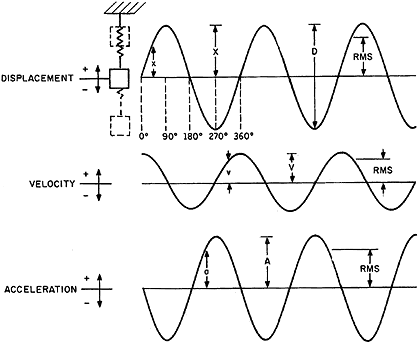 Figure 1. Phase relationships among displacement, velocity, and acceleration are shown on these time history plots. Figure 1. Phase relationships among displacement, velocity, and acceleration are shown on these time history plots. |
Velocity is defined as the time rate of change of displacement; acceleration is the time rate of change of velocity. Some technical disciplines use the term jerk to denote the time rate of change of acceleration.
Sinusoidal Motion Equation. The single-degree-of-freedom spring mass system, in forced vibration, maintained at a constant displacement amplitude, exhibits simple harmonic motion, or sinusoidal motion. That is, its displacement amplitude vs. time traces out a sinusoidal curve. Given a peak displacement of X, frequency f, and instantaneous displacement x:
| | (2) |
at any time, t.
Velocity Equation. Velocity is the time rate of change of displacement, which is the derivative of the time function of displacement. For instantaneous velocity, v:
| | (3) |
Since vibratory displacement is most often measured in terms of peak-to-peak, double amplitude, displacement D = 2X:
| | (4) |
If we limit our interest to the peak amplitudes and ignore the time variation and phase relationships:
| | (5) |
where:
V = peak velocity
Acceleration Equation. Similarly, acceleration is the time rate of change of velocity, the derivative of the velocity expression:
| | (6) |
and
| | (7) |
where:
A = peak acceleration
It thus can be shown that:
V = ![]() fD
fD
A = 2![]() 2 f2 D
2 f2 D
D = V/![]() f
f
D = A/2![]() 2 f2
2 f2
From these equations, it can be seen that low-frequency motion is likely to exhibit low-amplitude accelerations even though displacement may be large. It can also be seen that high-frequency motion is likely to exhibit low-amplitude displacements, even though acceleration is large. Consider two examples:
• At 1 Hz, 1 in. pk-pk displacement is only ~0.05 g acceleration; 10 in. is ~0.5 g • At 1000 Hz, 1g acceleration is only ~0.00002 in. displacement; 100 g is ~0.002 in.
Measuring Vibratory Displacement
Optical Techniques. If displacement is large enough, as at low frequencies, it can be measured with a scale, calipers, or a measuring microscope. At higher frequencies, displacement measurement requires more sophisticated optical techniques.
High-speed movies and video can often be used to measure displacements and are especially valuable for visualizing the motion of complex structures and mechanisms. The two methods are limited by resolution to fairly large displacements and low frequencies. Strobe lights and stroboscopic photography are also useful when displacements are large enough, usually >0.1 in., to make them practical.
The change in intensity or angle of a light beam directed onto a reflective surface can be used as an indication of its distance from the source. If the detection apparatus is fast enough, changes of distance can be detected as well.
The most sensitive, accurate, and precise optical device for measuring distance or displacement is the laser interferometer (see Figure 2).
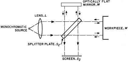 Figure 2. Interference patterns are created on the screen of the laser interferometer and can be related to displacement of the workpiece. Figure 2. Interference patterns are created on the screen of the laser interferometer and can be related to displacement of the workpiece. |
With this apparatus, a reflected laser beam is mixed with the original incident beam. The interference patterns formed by the phase differences can measure displacement down to <100 nm. NIST and other national primary calibration agencies use laser interferometers for primary calibration of vibration measurement instruments at frequencies up to 25 kHz.
Electromagnetic and Capacitive Sensors. Another important class of noncontact, special-purpose displacement sensors is the general category of proximity sensors. These are probes that are typically built into machinery to detect the motion of shafts inside journal bearings or the relative motion of other machine elements. The sensors measure relative distance or proximity as a function of either electromagnetic or capacitive (electrostatic) coupling between the probe and the target. Because these devices rely on inductive or capacitive effects, they require an electrically conductive target. In most cases, they must be calibrated for a specific target and specific material characteristics in the gap between probe and target.
Electromagnetic proximity sensors are often called eddy current probes because one of the most popular types uses eddy currents generated in the target as its measurement mechanism. More accurately, this type of sensor uses the energy dissipated by the eddy currents. The greater the distance from probe to target, the less electromagnetic coupling, the lower the magnitude of the eddy currents, and the less energy they drain from the probe. Other electromagnetic probes sense the distortion of an electromagnetic field generated by the probe and use that measurement to indicate the distance from probe to target.
Capacitive proximity sensor systems measure the capacitance between the probe and the target and are calibrated to convert the capacitance to distance. Capacitance is affected by the dielectric properties of the material in the gap as well as by distance, so calibration can be affected by a change of lubricant or contamination of the lubricant in a machine environment.
Contact Techniques. A variety of relative motion sensors use direct contact with two objects to measure relative motion or distance between them. These include LVDTs, cable position transducers (stringpots), and linear potentiometers. All of these devices depend on mechanical linkages and electromechanical transducers.
Seismic Displacement Transducers. These devices, discussed in detail later, were once popular but now are seldom used. They tend to be large, heavy, and short lived.
Double Integration of Acceleration. With the increasing availability and decreasing cost of digital signal processing, more applications are using the more rugged and more versatile accelerometers as sensors, then double integrating the acceleration signal to derive displacements. While older analog integration techniques tended to be noisy and inaccurate, digital processing can provide quite high-quality, high-accuracy results.
Measuring Vibratory Velocity
Transducers. Some of the earliest "high-frequency" vibration measurements were made with electrodynamic velocity sensors. These are a type of seismic transducer that incorporates a magnet supported on a soft spring suspension system to form the seismic (spring mass) system. The magnetic member is suspended in a housing that contains one or more multiturn coils of wire. When the housing is vibrated at frequencies well above the natural frequency of the spring mass system, the mass (magnet) is isolated from the housing vibration. Thus, the magnet is essentially stationary and the housing, with the coils, moves past it at the velocity of the structure to which it is attached. Electrical output is generated proportional to the velocity of the coil moving through the magnetic field. Velocity transducers are used from ~10 Hz up to a few hundred Hz. They tend to be large and heavy, and eventually wear and produce erratic outputs.
Laser Vibrometers. Laser vibrometers or laser velocimeters are relatively new instruments capable of providing high sensitivity and accuracy. They use a frequency-modulated (typically around 44 MHz) laser beam reflected from a vibrating surface. The reflected beam is compared with the original beam and the Doppler frequency shift is used to calculate the velocity of the vibrating surface. Alignment and standoff distance are critical. Because of the geometric constraints on location, alignment, and distances, they are limited to laboratory applications. One version of laser vibrometer scans the laser beam across a field of vision, measuring velocity at each point. The composite can then be displayed as a contour map or a colorized display. The vibration map can be superimposed on a video image to provide the maximum amount of information about velocity variations on a large surface.
Integration of Acceleration. As with displacement measurements, low-cost digital signal processing makes it practical to use rugged, reliable, versatile accelerometers as sensors and integrate their output to derive a velocity signal.
Measuring Vibratory Acceleration
Most modern vibration measurements are made by measuring acceleration. If velocity or displacement data are required, the acceleration data can be integrated (velocity) or double integrated (displacement). Some accelerometer signal conditioners have built-in integrators for that purpose. Accelerometers (acceleration sensors, pickups, or transducers) are available in a wide variety of sizes, shapes, performance characteristics, and prices. The five basic transducer types are servo force balance; crystal-type or piezoelectric; piezoresistive or silicon strain gauge type; integral electronics piezoelectric; and variable capacitance. Despite the different electromechanical transduction mechanisms, all use a variation of the spring mass system, and are classified as seismic transducers.
Seismic Accelerometer Principle. All seismic accelerometers use some variation of a seismic or proof mass suspended by a spring structure in
 |
Accelerometers. Transducers designed to measure vibratory acceleration are called accelerometers. There are many varieties including strain gauge, servo force balance, piezoresistive (silicon strain gauge), piezoelectric (crystal-type), variable capacitance, and integral electronic piezoelectric. Each basic type has many variations and trade names. Most manufacturers provide excellent applications engineering assistance to help the user choose the best type for the application, but because most of these sources sell only one or two types, they tend to bias their assistance accordingly.
For most applications, my personal bias is toward piezoelectric accelerometers with internal electronics. The primary limitation of these devices is temperature range. Although they exhibit low-frequency roll-off, they are available with extremely low-frequency capabilities. They provide a preamplified low-impedance output, simple cabling, and simple signal conditioning, and generally have the lowest overall system cost.
Most important to the user are the performance and environmental specifications and the price. What's inside the box is irrelevant if the instrument meets the requirements of the application, but when adding to existing instrumentation it is important to be sure that the accelerometer is compatible with the signal conditioning. Each type of accelerometer requires a different type of signal conditioning.
Accelerometer Types. The most common seismic transducers for shock and vibration measurements are:
- Piezoelectric (PE); high-impedance output
- Integral electronics piezoelectric (IEPE); low-impedance output
- Piezoresistive (PR); silicon strain gauge sensor
- Variable capacitance (VC); low-level, low-frequency
- Servo force balance
Piezoelectric (PE) sensors use the piezoelectric effects of the sensing element(s) to produce a charge output. Because a PE sensor does not require an external power source for operation, it is considered self-generating. The "spring" sensing elements provide a given number of electrons proportional to the amount of applied stress (piezein is a Greek word meaning to squeeze). Many natural and man-made materials, mostly crystals or ceramics and a few polymers, display this characteristic. These materials have a regular crystalline molecular structure, with a net charge distribution that changes when strained [1].
Piezoelectric materials may also have a dipole (which is the net separation of positive and negative charge along a particular crystal direction) when unstressed. In these materials, fields can be generated by deformation from stress or temperature, causing piezoelectric or pyroelectric output, respectively. The pyroelectric outputs can be very large unwanted signals, generally occurring over the long time periods associated with most temperature changes [1]. Polymer PE materials have such high pyroelectric output that they were originally used as thermal detectors. There are three pyroelectric effects, which will be discussed later in detail.
Charges are actually not "generated," but rather just displaced. (Like energy and momentum, charge is always conserved.) When an electric field is generated along the direction of the dipole, metallic electrodes on faces at the opposite extremes of the gradient produce mobile electrons that move from one face, through the signal conditioning, to the other side of the sensor to cancel the generated field. The quantity of electrons depends on the voltage created and the capacitance between the electrodes [1]. A common unit of charge from a PE accelerometer is the picocoulomb, or 10-12 coulomb, which is something over 6 × 10⁶ electrons.
Choosing among the many types of PE materials entails a tradeoff among charge sensitivity, dielectric coefficient (which, with geometry, determines the capacitance), thermal coefficients, maximum temperature, frequency characteristics, and stability. The best S/N ratios generally come from the highest piezoelectric coefficients.
Naturally occurring piezoelectric crystals such as tourmaline or quartz generally have low-charge sensitivity, about one-hundredth that of the more commonly used ferroelectric materials. (But these low-charge output materials are typically used in the voltage mode, which will be discussed later.) Allowing smaller size for a given sensitivity, ferroelectric materials are usually man-made ceramics in which the crystalline domains (i.e., regions in which dipoles are naturally aligned) are themselves aligned by a process of artificial polarization.
Polarization usually occurs at temperatures considerably higher than operating temperatures to speed the process of alignment of the domains. Depolarization, or relaxation, can occur at lower temperatures, but at very much lower rates, and can also occur with applied voltages and preload pressures. Depolarization always results in temporary or permanent loss of sensitivity. Tourmaline, a natural crystal that does not undergo depolarization, is particularly useful at very high temperatures.
Because they are self-generating, PE transducers cannot be used to measure steady-state accelerations or force, which would put a fixed amount of energy into the crystal (a one-way squeeze) and therefore a fixed number of electrons at the electrodes. Conventional voltage measurement would bleed electrons away, as does the sensor's internal resistance. (High temperature or humidity in the transducer would exacerbate the problem by reducing the resistance value.) Energy would be drained and the output would decay, despite the constant input acceleration/force [1].
External measurement of PE transducer voltage output requires special attention to the cable's dynamic behavior as well as the input characteristics of the preamplifier. Since cable capacitance directly affects the signal amplitude, excessive movement of the cable during measurement can cause changes in its capacitance and should be avoided. Close attention should also be paid to the preamp's input impedance; this should be on the order of 1000 M![]() or higher to ensure sufficient low-frequency response.
or higher to ensure sufficient low-frequency response.
In practice, a charge amplifier is normally used with a PE transducer (see Figure 4).
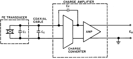 Figure 4. The feedback capacitance of the charge converter determines the ratio of output voltage to input charge of a charge amplifier. Figure 4. The feedback capacitance of the charge converter determines the ratio of output voltage to input charge of a charge amplifier. |
Instead of measuring voltage externally, a charge should be measured with a charge converter. It is a high-impedance op amp with a capacitor as its feedback. Its output is proportional to the charge at the input and the feedback capacitor, and is nearly unaffected by the input capacitance of the transducer or attached cables. The high-pass corner frequency is set by the feedback capacitor and resistor in a charge converter, and not the transducer characteristics. (The transducer resistance changes noise characteristics, not the frequency.) If time constants are long enough, the AC-coupled transducer will suffice for most vibration measurements.
Perhaps the most important limitation of high-impedance output PE transducers is that they must be used with "noise-treated" cables; otherwise, motion in the cable can displace triboelectric charge, which adds to the charge measured by the charge converter. Triboelectric noise [2,3] is a common source of error found in typical coaxial cables.
Most PE transducers are extremely rugged. Each of the various shapes and sizes available comes with its own performance compromises. The most common types of this transducer are compression and shear designs. Shear design offers better isolation from environmental effects such as thermal transient and base strain, and is generally more expensive. Beam-type design, a variation of the compression design, is also quite popular due to its lower manufacturing cost. But beam design is generally more fragile and has limited bandwidth [3].
Integral Electronics Piezoelectric (IEPE). Many piezoelectric accelerometers/force transducers include integral miniature hybrid amplifiers, which, among their other advantages, do not need noise-treated cable. Most require an external constant current power source. Both the input supply current and output signal are carried over the same two-wire cable. The low-impedance output of the IEPE design (see Figure 5) provides relative immunity to the effects of poor cable insulation resistance, triboelectric noise, and stray signal pickup [5,6,7].
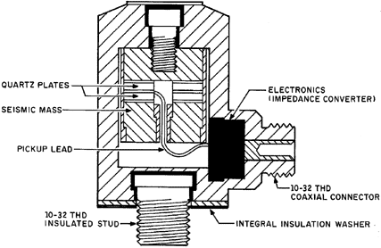 Figure 5. This IEPE accelerometer has an inverted compression seismic system and an electronic module in the connector. Figure 5. This IEPE accelerometer has an inverted compression seismic system and an electronic module in the connector. |
Output-to-weight ratio of IEPE is higher than with PE transducers. Additional functions can be incorporated into the electronics (see Figure 6), including filters, overload protection, and self-identification.
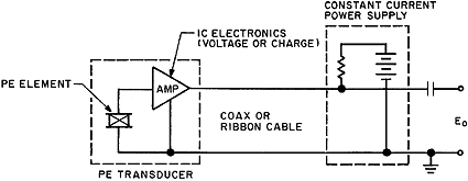 Figure 6. The IEPE accelerometer system provides a constant current source for the internal amplifier and a capacitor to block the DC bias of the output signal. Figure 6. The IEPE accelerometer system provides a constant current source for the internal amplifier and a capacitor to block the DC bias of the output signal. |
Lower cost cable and conditioning can be used since the conditioning requirements are comparatively lax compared to PE or PR. The sensitivity of IEPE accelerometers/force transducers, in contrast to PR, is not significantly affected by supply changes. Instead, dynamic range, the total possible swing of the output voltage, is affected by bias and compliance voltages. Only with large variations in current supply would there be problems with frequency response when driving high-capacitance loads [8].
A disadvantage of built-in electronics is that it generally limits the transducer to a narrower temperature range. In comparison with an identical transducer design that does not have internal electronics, the high-impedance version will always have a higher mean time between failures (MTBF) rating. In addition, the necessarily small size of the amplifier may preclude some of the desirable features offered by a full-blown laboratory amplifier, such as the ability to drive long cable. Slew limiting is therefore a concern with these transducers (some designs have relatively high output impedance) when driving long lines or other capacitive loads. The problem can be remedied by increasing the amount of drive current within the limit specified by the manufacturer [8].
The circuits need not necessarily be charge converters because the capacitance due to leads between the sensor and the amplifier is small and well controlled. Quartz is used in the voltage mode, i.e., with source followers, because its small dielectric coefficient provides comparatively high voltage per unit charge. Voltage conversion also aids ferroelectric ceramics that have the sag in frequency response in charge mode due to their frequency-dependent dielectric coefficient. The amplitude frequency response in the voltage mode is quite flat.
Piezoresistive. A PR accelerometer is a Wheatstone bridge of resistors incorporating one or more legs that change value when strained. Because the sensors are externally supplied with energy, the output can be meaningfully DC coupled to respond to steady-state conditions. Data on steady-state accelerations comes at a cost, however. The sensitivity of a bridge varies almost directly with the input excitation voltage, requiring a highly stable and quiet excitation supply [9,10].
The output of a bridge configuration is the difference between the two output leads. A differential amplifier is required or, alternatively, both leads from the excitation must float to allow one of the output lines to be tied to ground. The differential configuration provides the advantage of common-mode rejection; that is to say, any noise signals picked up on the output lines, if equal, will be canceled by the subtraction in the amplifier.
A cautionary note is in order here: With high-output PR transducers, there is a temptation to dispense with an amplifier and simply to connect the output leads directly to an oscilloscope. This will not work if both the scope and the excitation are single ended. Oscilloscopes often have single-ended input (the negative side of the input is ground). If the excitation is also grounded (with the excitation equal to ground), one leg of the bridge is shunted and the entire excitation voltage is placed across that one leg of the bridge. If you are using AC coupling on the scope, you might misinterpret the reasonably shaped, but small and noisy, output.
Most PR sensors use two or four active elements. Voltage output of a two-arm, or half-bridge, sensor is half that of a four-arm, or full bridge.
Stability requirements for a PR transducer power supply and its conditioning are considerably tighter than they are for IEPE. Low-impedance PR transducers share the advantages of noise immunity provided by IEPE, although the output impedance of PR is often large enough that it cannot drive large capacitive loads. As is the case with an underdriven IEPE, the result is a low-pass filter on the output, limiting high-frequency response.
The sensitivity of a strain gauge comes from both the elastic response of its structure and the resistivity of the material. Wire and thick or thin film resistors have low gauge factors; that is, the ratio of resistance change to the strain is small. Their response is dominated by the elastic response. They are effectively homogeneous blocks of material with resistivity of nearly constant value. As with any resistor, they have a value proportional to length and inversely proportional to cross-sectional area. If a conventional material is stretched, its width reduces while the length increases. Both effects increase resistance.
The Poisson ratio defines the amount a lateral dimension is narrowed compared to the amount the longitudinal dimension is stretched. Given a Poisson ratio of 0.3 (a common value), the gauge factor would be 1.6; resistance would change 1.6 × more than it is strained. A typical gauge factor for metal strain gauges is ~2.
The response of strain gauges with higher gauge factors is dominated by the piezoresistive effect, which is the change of resistivity with strain. Semiconductor materials exhibit this effect, which, like piezoelectricity, is strongly a function of crystal orientation. Like other semiconductor properties, it is also a strong function of dopant concentration and temperature. Gauge factors near 100 are common for silicon gauges, and, when combined with small size and the stress-concentrating geometries of anisotropically etched silicon, the efficiency of the silicon PR transducer is very impressive. The miniaturization allows natural frequencies >1 MHz in some PR shock accelerometers.
Most contemporary PR sensors are manufactured from a single piece of silicon. In general, the advantages of sculpting the whole sensor from one homogeneous block of material are better stability, less thermal mismatch between parts, and higher reliability [11]. Underdamped PR accelerometers tend to be less rugged than PE devices. Single-crystal silicon can have extraordinary yield strength, particularly with high strain rates, but it is a brittle material nonetheless. Internal friction in silicon is very low, so resonance amplification can be higher than for PE transducers. Both these features contribute to its comparative fragility, although if properly designed and installed they are used with regularity to measure shocks well above 100,000 g. They generally have wider bandwidths than PE transducers (comparing models of similar full-scale range), as well as smaller nonlinearities, zero shifting, and hysteresis characteristics. Because they have DC response, they are used when long-duration measurements are to be made.
In a typical monolithic silicon sensing element of a PR accelerometer, the 1 mm square silicon chip incorporates the entire spring, mass, and four-arm PR strain gauge bridge assembly. The sensor is made from a single-crystal silicon by means of anisotropic etching and micromachining techniques. Strain gauges are formed by a pattern of dopant in the originally flat silicon. Subsequent etching of channels frees the gauges and simultaneously defines the masses as simply regions of silicon of original thickness.
The bridge circuit can be balanced by placing compensation resistor(s) in parallel or series with any of the legs, correcting for the matching of either the resistance values and/or the change of the values with temperature. Compensation is an art; because the PR transducer can have nonlinear characteristics, it is inadvisable to operate it with excitation different from the conditions under which it was manufactured or calibrated [12]. For example, PR sensitivity is only approximately proportional to excitation, which is usually a constant voltage or, in some cases, constant current, which has some performance advantages [13]. Because thermal performance will in general change with excitation voltage, there is not a precise proportionality between sensitivity and excitation. Another precaution in dealing with voltage-driven bridges, particularly those with low resistance, is to verify that the bridge gets the proper excitation. The series resistance of the input lead wires acts as a voltage divider. Take care that the input lead wires have low resistance, or that a six-wire measurement be made (with sense lines at the bridge to allow the excitation to be adjusted) so the bridge gets the proper excitation.
Constant current excitation does not have this problem with series resistance. However, PR transducers are generally compensated assuming constant voltage excitation and might not give the desired performance with constant current. The balance of the PR bridge is its most sensitive measure of health, and is usually the dominant feature in the total uncertainty of the transducer. The balance, sometimes called bias, zero offset, or ZMO (zero measurand output, the output with 0 g), can be changed by several effects that are usually thermal characteristics or internally or externally induced shifts in strains in the sensors. Transducer case designs attempt to isolate the sensors from external strains such as thermal transients, base strain, or mounting torque. Internal strain changes, e.g., epoxy creep, tend to contribute to long-term instabilities. All these generally low-frequency effects are more important for DC transducers than for AC-coupled devices because they occur more often in the wider frequency band of the DC-coupled transducer.
Some PR designs, particularly high-sensitivity transducers, are designed with damping to extend frequency range and overrange capability. Damping coefficients of ~0.7 are considered ideal. Such designs often use oil or some other viscous fluid. Two characteristics dictate that the technique is useful only at relatively low frequencies: damping forces are proportional to flow velocity, and adequate flow velocity is attained by pumping the fluid with large displacements. This is a happy coincidence for sensitive transducers in that they operate at the low acceleration frequencies where displacements are adequately large. Viscous damping can effectively eliminate resonance amplification, extend the overrange capability, and more than double the useful bandwidth. However, because the viscosity of the damping fluid is a strong function of temperature, the useful temperature range of the transducer is substantially limited.
Variable Capacitance. VC transducers are usually designed as parallel-plate air gap capacitors in which motion is perpendicular to the plates. In some designs the plate is cantilevered from one edge, so motion is actually rotation; other plates are supported around the periphery, as in a trampoline. Changes in capacitance of the VC elements due to acceleration are sensed by a pair of current detectors that convert the changes into voltage output. Many VC sensors are micromachined as a sandwich of anisotropically etched silicon wafers with a gap only a few microns thick to allow air damping. The fact that air viscosity changes by just a few percent over a wide operating temperature range provides a frequency response more stable than is achievable with oil-damped PR designs.
In a VC accelerometer, a high-frequency oscillator provides the necessary excitation for the VC elements. Changes in capacitance are sensed by the current detector. Output voltage is proportional to capacitance changes, and, therefore, to acceleration. The incorporation of overtravel stops in the gap can enhance ruggedness in the sensitive direction, although resistance to overrange in transverse directions must rely solely on the strength of the suspension, as is true of all other transducer designs without overtravel stops. Some designs can survive extremely high acceleration overrange conditions-as much as 1000 × full-scale range [14].
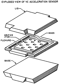 |
The sensor of a typical micromachined VC accelerometer is constructed of three silicon elements bonded together to form a hermetically sealed assembly (see Figure 7). Two of the elements are the electrodes of an air dielectric, parallel-plate capacitor. The middle element is chemically etched to form a rigid central mass suspended by thin, flexible fingers. Damping characteristics are controlled by gas flow in the orifices located on the mass.
VC sensors can provide many of the best features of the transducer types discussed earlier: large overrange, DC response, low-impedance output, and simple external signal conditioning. Disadvantages are the cost and size associated with the increased complexity of the onboard conditioning. Also, high-frequency capacitance detection circuits are used, and some of the high-frequency carrier usually appears on the output signal. It is generally not even noticed, being up to three orders of magnitude (i.e., 1000 ×) higher in frequency than the output signals.
Servo (Force Balance). Although servo accelerometers are used predominantly in inertial guidance systems, some of their performance characteristics make them desirable in certain vibration applications. All the accelerometer types described previously are open-loop devices in which the output due to deflection of the sensing element is read directly. In servo-controlled, or closed-loop, accelerometers, the deflection signal is used as feedback in a circuit that physically drives or rebalances the mass back to the equilibrium position. Servo accelerometer manufacturers suggest that open-loop instruments that rely on displacement (i.e., straining of crystals and piezoresistive elements) to produce an output signal often cause nonlinearity errors. In closed-loop designs, internal displacements are kept extremely small by electrical rebalancing of the proof mass, minimizing nonlinearity. In addition, closed-loop designs are said to have higher accuracy than open-loop types. However, definition of the term accuracy varies. Check with the sensor manufacturer.
Servo accelerometers (see Figure 8) can take either of two basic geometries: linear (e.g., loudspeaker) and pendulous (meter movement).
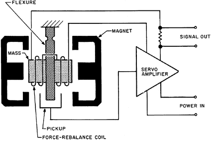 Figure 8. The servo force balance accelerometer produces an output proportional to the force required to maintain the mass in an equilibrium position. Figure 8. The servo force balance accelerometer produces an output proportional to the force required to maintain the mass in an equilibrium position. |
Pendulous geometry is most widely used in commercial designs. Until recently, the servo mechanism was primarily based on electromagnetic principles. Force is usually provided by driving current through coils on the mass in the presence of a magnetic field. In the pendulous servo accelerometer with an electromagnetic rebalancing mechanism, the pendulous mass develops a torque proportional to the product of the proof mass and the applied acceleration. Motion of the mass is detected by the position sensors (typically capacitive sensors), which send an error signal to the servo system. The error signal triggers the servo amplifier to output a feedback current to the torque motor, which develops an opposing torque equal in magnitude to the acceleration-generated torque from the pendulous mass. Output is the applied drive current itself (or across an output resistor), which, analogous to the deflection in the open-loop transducers, is proportional to the applied force and therefore to the acceleration.
In contrast to the rugged spring elements of the open-loop transducers, the rebalancing force in the case of the closed-loop accelerometer is primarily electrical and exists only when power is provided. The springs are as flimsy in the sensitive direction as feasible and most damping is provided through the electronics. Unlike other DC-response accelerometers whose bias stability depends solely on the characteristics of the sensing element(s), it is the feedback electronics in the closed-loop design that controls bias stability. Servo accelerometers therefore tend to offer less zero drifting, which is the major reason for their uses in vibration measurements. In general, they have a useful bandwidth of <1000 Hz and are designed for use in applications with comparatively low acceleration levels and extremely low frequency components.
Part 2 of this article, which will appear in the March issue of Sensors, will address the criteria that should be considered when selecting a vibration measurement system.
References
1. A. Chu. "Zero Shift of Piezoelectric Accelerometers in Pyroshock Measurements," Endevco TP No. 293.
2. "Shock & Vibration Measurement Technology." 1987. Endevco.
3. "Measuring Vibration." 1982. Bruel & Kjaer.
4. C. Harris. 1995. Shock and Vibration Handbook, 4th Ed., McGraw Hill.
5. "General Guide to ICP Instrumentation." March 1973. PCB Piezotronics, #G-0001.
6. "Introduction to Piezoelectric Sensors." March 1985. PCB Piezotronics, #018.
7. "Application of Integrated-Circuit Electronics to Piezoelectric Transducers." March 1967. PCB Piezotronics, #G-01.
8. "Isotron Instruction Manual." 1995. Endevco, IM 31704.
9. "Instruction Manual for Endevco Piezoresistive Accelerometers." 1978. Endevco, #121.
10. "Entran Accelerometer Instruction and Selection Manual." 1987. Entran Devices.
11. R. Sill. "Testing Techniques Involved with the Development of High Shock Acceleration Sensors." Endevco, TP 284.
12. R. Sill. "Minimizing Measurement Uncertainty in Calibration and Use of Accelerometers." Endevco, TP 299.
13. P.K. Stein. "The Constant Current Concept for Dynamic Strain Measurement." Stein Engineering Services, Inc., Lf/MSE Publication 46.
14. B. Link. "Shock and Vibration Measurement Using Variable Capacitance." Endevco, TP 296.