
While both magnetoresistive and integrated Hall sensors measure the strength of magnetic field components, they do so in different ways and this can directly affect their successful use in a position sensing application. Choosing which of the two is a better fit for your application may require you to consider sensor characteristics that don't show up on manufacturers' data sheets. This article is designed to help your decision process by reviewing two angle sensors—an anisotropic magnetoresistive (AMR) sensor and a Hall sensor—in a position-sensing application example.
The Theoretical Basics
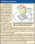
Figure 1 shows how the two sensor types react in the presence of an external magnetic field. A magnetoresistive (MR) sensor records axis or magnet angle information via the field vector in the chip plane. The AMR effect is a "resistor" effect based on the dependence of electrical resistance on the angle between the directions of the current flow and magnetization of a ferromagnetic material. An external magnetic field can switch the internal direction of magnetization of the AMR material and thus effect changes in resistance (ΔR/R) that are typically on the order of a few percent.
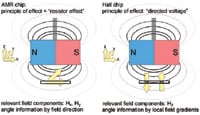 Figure 1. Here we see the basic principles of operation for AMR and Hall effect sensors. |
Several resistors connected in a Wheatstone bridge are used to measure angles. Each component resistor contributes to a change in the differential output voltage of the bridge, depending on the X,Y field direction in the sensor plane and on the direction of current flow in the resistors. This direction of current flow is either given by the alignment of the resistor paths or is forced in another direction by short-circuit contacts (barber poles).
For our sample AMR sensor (see its specifications in Figure 2), the bridge provides a differential sine voltage of 70 mV with a cyclic repetition every 180°. A field aligned in the opposite direction produces the same resistive effect.
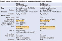 Figure 2. Selected electrical characteristics of the sensors from the manufacturers' data sheets. |
To evaluate this bridge voltage we need a useful reference—preferably a reference voltage. Ideally, this is a second bridge set at a tilt to the first bridge and generating a differential cosine voltage. We can now determine the angle to be measured from the relationship between the two bridge voltages. Since any change in sensitivity (caused by temperature, for example) will affect both voltages in a similar way, these changes are not important for determining the angle.
For our sample Hall sensor, we're interested in the field component vertical to the chip. The Hall effect generates a directed voltage, typically of just a few millivolts, which is dependent on the strength of the Z component of a magnetic field. Consequently, a single Hall element sees only the distance between itself and the magnet. If several elements are used, each recording the Z field at various positions, then evaluating local gradients provides information on the angle. The arrangement of Hall elements on the chip determines which magnet to use since the sensor must be able to detect the bent near magnetic field. External homogenous stray fields, such as those from brushless DC motor assemblies, cannot cause interference.
Because the polarity of the Hall voltage follows the field direction, a magnetic north pole can be distinguished from a south pole. The range of angle measurement is extended to 360° but with half the sensitivity for angle changes within 180° in comparison to MR sensors.
To summarize, a designer can expect the following characteristics from the two types of sensors:
For the AMR sensor:
- 1. High sensitivity and a low-noise signal.
- 2. A large operating distance from the magnet is possible.
- 3. Angle of measurement is up to 180° but with higher angle sensitivity.
- 4. Possible disturbance from external stray fields.
For the Hall sensor:
- 1. Because of internal preamplification, sensitivity is comparable.
- 2. Sensor functions only in the near field of the magnet.
- 3. Angle of measurement is up to 360°.
- 4. Possible disturbance from external stray "dipole fields."
Comparing Sensor Specifications
For our experiment, the two sample sensors are the KMZ43T MR angle sensor from Philips and the iC-MA Hall sensor from iC-Haus.
We shall exclude the various integrated evaluation functions of the Hall sensor from this study (for further discussion see sidebar "iC-MA Sensor Functions") and concentrate instead on the analog sensor signals which have been preconditioned on the chip. In the experiment these analog signals are linked to the evaluation circuitry.
Manufacturers' data sheets, as shown in Figure 2, don't usually specify the quality of the analog sine/cosine sensor signals with respect to harmonic-free waveform, amplitude synchronism, phase precision, and offset nor do they entirely specify changes in field strength dependency or temperature. The information provided is, however, sufficient to let us adapt the evaluation circuitry to the sensor and to correct first-order signal errors.
We want a reasonable signal level. The MR sensor's typical signal amplitude of 70 mV requires preamplification; in contrast, the Hall sensor provides preamplification on chip. Nonmatching amplitudes are not acceptable: a difference between the sine and cosine signal amplitude causes an angle error of ~0.2° (with respect to the signal period) at a difference in amplitudes of 0.7%. While the MR sensor does not suffer from nonmatching amplitudes, the Hall sensor will need to be calibrated due to the 5% signal-referenced specification.
Calibration of the offset is even more important because as little as a 1% error for both the sine and cosine signal leads to an angle error of ~0.8° (with respect to the signal period). The offset of the MR sensor is considerably higher than that of the Hall sensor, which is already conditioned on the chip. For more precise angle measurements both sensors will require additional offset calibration.
Change in offset voltage with temperature is also relevant to the angle error. With the MR sensor, an assessment based on drift values produces a signal-referenced change of 0.3% across 100 K, thus marking out error margins. Unless we compensate for the drift with the evaluation circuitry, the angle error must lie within these margins. With the Hall sensor, information on drift is not directly available. We narrow down the drift values based on the specifications governing system accuracy which include those for the on-chip interpolator. Since the sensor error is <0.5°, the provided interpolation resolution of 6 to 8 bits (1.4° angle error at 8-bit resolution) is too crude and exceeds the achievable resolution of the analog Hall signals.
Rather than study the electrical characteristics of the individual parts, it's more useful to assess the overall system, including the designated evaluation circuitry. Measuring the absolute angle error against a reference system should tell us how both sensor types behave in a magnetic field when assembled with typical mechanical tolerances. According to the data sheets the sensors should tolerate alignment variation of several tenths of a millimeter with respect to the center of the magnet axis.
Angle Error Measuring Setup
As a reference system for measuring angle error, a high-precision optical absolute encoder used in our experimental setup provided an absolute angle accuracy of better than 50 arc-seconds and at the same time acted as a mechanical base for the drive and magnet (see Figure 3).
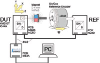 Figure 3. Here's a diagram of the experimental setup. The reference encoder's axis, holding the magnet, was belt-driven smoothly from a gearbox DC motor. All measurements were taken over at least three full turns. |
An adjustable stage bearing the interpolator card with the MR or Hall sensor device under test (DUT) was placed opposite the encoder. Evaluation electronics consisted of an iC-NQ 13-bit sine-to-digital converter that uses the BiSS Interface as a fast data output and calibration interface.
The BiSS Interface enables the synchronously triggered acquisition of measurement data for several devices at once. We therefore chose a sine/cosine encoder as a reference, mapped onto the BiSS Interface using a second iC-NQ interpolator. As the reference encoder provides 2048 sine cycles per revolution, a low interpolation factor was sufficient.
All settings were made directly from a PC; Figure 4 gives a summary of these. As expected, the Hall sensor had to be adjusted with regard to the difference in amplitude (parameter RATIO) and offset (parameter SINOFFS), while the main adjustments to the MR sensor were made to its offset (parameter SINOFFS).
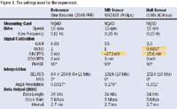 Figure 4. The settings used for the experiment. |
Measurement Results
For both sensors we used an interpolator resolution of 10 bits or 1024 angle steps so that all measurement data could be subjected to the same graphic evaluation using Matlab. This allowed us to make a direct comparison between the angle error curves using a Y scale marked in LSB (1 LSB = 360°/1024 = 0.35°).
A 4 mm diameter, diametrically magnetized NdFeB magnet was used. Even when ideally placed in relation to the magnet on all three axes both sensors initially demonstrated large deviations in angle while the sensor signals remained uncalibrated (shown as the red curves in Figure 5). Once the signal errors had been eliminated, using the settings in Figure 4, the minimum error level, shown as a green curve, was achieved. This minimum error curve is given as a "green" reference in all ensuing figures.
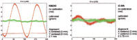 Figure 5. Here we see the measurement results for the MR sensor on the left and the Hall effect sensor on the right. The graph shows both uncalibrated (red line) and calibrated (green line) results. |
We then tried to discover whether the two sensor types make differing demands on the mechanical adjustment because of their different principles of measurement. We noted several error curves and added tolerances axis by axis.
With respect to the Z axis, the operating distance from the magnet shown in Figure 6 reveals that both sensors permit tolerances within the millimeter range without overshooting an angle error threshold of 0.5°. As expected, the MR sensor permits a greater operating distance.
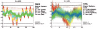 Figure 6. This graph shows the measurement results for the MR sensor (left) and Hall effect sensor (right) when the magnet was displaced by various amounts. |
Due to the finer scaling of the Y axis we can see that the MR sensor's error curve has the lower fluctuation which can be explained by its higher basic resolution and double signal period. We can achieve an equivalent result for the Hall sensor by raising the resolution of the interpolator to 11 bits (shown as the blue curve in Figure 6B); the signal is then still visible above the noise level.
A misalignment on the X,Y plane causes a larger error than a change in operating distance (see Figure 7). The Hall sensor experienced an angle error of up to 1° or 3 LSB when the center of the axis was moved diagonally 0.2 mm (X and Y axes). Even a purely horizontal (X axis) or purely vertical (Y axis) shift can generate a similar error which does not have to look completely symmetrical. Under the same conditions the MR sensor had a maximum error of ~0.7° or 2 LSB, with the chosen magnet well-suited to the small sensor area.
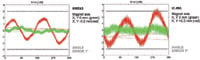 Figure 7. Here we see the measurement results when the sensors are misaligned on the X,Y plane. |
The adjustment tolerance mentioned above is not a problem for low-angle resolutions; up to an angular resolution of 1.4° (8 bits) the angle error remains lower than the LSB. For higher resolutions and levels of precision a finer adjustment is required and the choice of magnet may also need to be optimized.
Another possible source of error is a tilted sensor, simulated in our setup by tilting the magnet axis. Even with a clearly visible tilt angle of 1.5° (φ in Figure 3) the angle error curve did not exceed a threshold of ±1 LSB when the sensor position was adjusted on the X,Y plane. Tilting within a certain margin is tolerated and in this respect the two sensors do not differ markedly.
Disturbance fields as possible sources of error were not explored in any detail. The influence of changes in temperature was examined within a range of –40°C to 60°C. Within this range, signal calibration at room temperature proved optimal. The early stages of drift effects were recognizable for the MR sensor from ~70°C upward. A separate investigation of a sensor system for high ambient temperatures, including the evaluation electronics, would undoubtedly be prudent.
Results and Considerations
Although in principle both sensors vary, in the angle sensor application described here the differences were surprisingly minor. This applies to both the permissible assembly tolerances and the angle measurement results. Major differences include the MR sensor's high incremental angle resolution and the Hall sensor's absolute angle resolution across 360°. The latter would prove useful for applications calling for low resolutions that the integrated sensor electronics can already provide. The required temperature range can also influence the choice of sensor, for example the MR sensor is suitable in principle for applications beyond the –40°C to 125°C range.
Future Prospects
Keep in mind that the sensing technology you choose is going to depend heavily on the specifics of the target application. This article has tackled various points for further discussion demonstrating the potential of both MR and Hall technologies. The future could prove exciting when new, higher-precision MR sensors operating at lower field strengths are brought onto the market. On request, integrated Hall sensors can already provide DSP; improvements in signal quality are also expected, as is improved user-friendliness.
 iC-MA Sensor Functions |
Links
iC-MA and iC-NQ data sheets: www.ichaus.com
KMZ43 data sheet: www.semiconductors.philips.com
MR sensor technology: www.sensitec.de, www.hl-planar.de
Joachim Quasdorf, Dipl.-Ing. can be reached at iC-Haus GmbH, Bodenheim, Germany; +49-6135-9292-300, [email protected], www.ichaus.com